Gravity Optimizer Math.md

Gravity Optimizer Math

Lets imagine an inclined plane and write some basic kinematic physics:

In this simple example lets forget the rolling part of the ball and focus on $a_L$. first we will calculate $\theta$ by using $dL$ and $dW$: Equation 1: $tan(\theta) = \frac{dL}{dW} \Rightarrow \theta = tan^{-1}(\frac{dL}{dW})$ from now on i call $\frac{dL}{dW}$ as $g$ which stands for gradient in this imaginary world there is a universal acceleration in L axis direction which is $a_L$. lets calculate relationship between inclined-plane's local coordinate system which is <x, y> and global coordinate system which is <W, L>. by using basic trigonometric relation we can achieve this as follow: Equation 2: $W=x.cos\theta \Rightarrow \Delta W=\Delta x.cos\theta$ Equation 3: $L=x.sin\theta \Rightarrow \Delta L=\Delta x.sin\theta$ now lets infer $a_x$: Equation 4: $a_x=-a_L.sin\theta$ in this situation that $a_L$ and $\theta$ does not change with time we can write constant acceleration equation for position as follow: Equation 5: $x=\frac{1}{2}.a_x.t^2+v_{0_x}.t+x_0$ by assuming $v_0$ is $0$ the new shape of equation 5 will be as below: Equation 6: $\Delta x = \frac{1}{2}.a_x.t^2$ and by substituting equation 6 into equation 2 we can write: Equation 7: $\Delta W = \frac{1}{2}.a_x.t^2 cos(\theta)$ plug $a_x$ from equation 4 in equation 7: Equation 8: $\Delta W = -\frac{1}{2}.a_L.t^2.cos(\theta).sin(\theta)$ equations for calculating sine and cosine of $tan^{-1}$ are as follow: Equation 9: $sin(tan^{-1}(x))=\frac{x}{\sqrt{1+x^2}}$ Equation 10: $cos(tan^{-1}(x))=\frac{1}{\sqrt{1+x^2}}$ now by using equations 1, 8, 9, 10 we can write: Equation 11: $\Delta W = -\frac{1}{2}.a_L.t^2.\frac{g}{1+g^2}$ Equation 11 is our raw parameter-update equation. but as you can see there is a lot of hyper-parameters in this equation which need a lot of time for tuning. beside that these hyper-parameters are not intuitive.

Learning Rate

we used to work with more familiar hyper-parameters like learning rate. so lets wrap up every hyper-parameter until now as a single one which is learning rate: Equation 12: $l=\frac{1}{2}.a_L.t^2$ then: Equation 13: $\Delta W = \frac{-lg}{1+g^2}$ this is more intuitive equation but it does not look so reasonable! how we can be sure about equation 12? is that really learning rate or just a name for an unknown hyper-parameter? lets look at optimization methods in different way. we can simplify all back-prop based optimization methods as a function of gradient. every optimization method gets gradient and calculate a step for parameter to take. for example vanilla Gradient Descent is a linear function of gradient: Equation 14: $\Delta W = -lg$ we can plot that as below: now lets plot gravity from Equation 13 in this plot and compare it to GD for a given value of learning rate: it is obvious from this plot that for small value of gradient Gravity behave like Gradient Descent. in math words $\lim_{g \to 0} Gravity(g) = GD(g)$. but how much small? lets try different learning rate and plot that too: in this plot we can see by changing learning rate the gradient at which maximum step occurs(i.e. Extremum) will not change. no matter what learning rate we choose, the maximum step always occurs at $g=1$ which corresponds to 45°.

Max-Step Grad

We need more control. so far only parameters we encounter are $a_L$ and $t$ which both of them are universal. by universal i mean they are same for every parameter in weight matrix. we want specific control on this particular parameter.well, say hello to Galileo Galilei. you probably heard the myth which states that Galileo had dropped balls from the Leaning Tower of Pisa to demonstrate that their time of descent was independent of their mass. While this story has been retold in popular accounts, there is no account by Galileo himself of such an experiment, and it is generally accepted by historians that it was at most a thought experiment which did not actually take place. However, most of his experiments with falling bodies were carried out using inclined planes where both the issues of timing and air resistance were much reduced. in fact inclined plane acts like a slow motion video recorded by a high speed camera. when you increase the angle $\theta$ the falling time will be reduced and everything happens quickly. in contrast by reducing $\theta$ we bend time and slow down ball's falling motion. we can do what Galileo did by changing $\theta$ in a way that help us to reach minimum of $L$ more quickly and without divergence. we will do this by tweaking gradient with a coefficient called $m$ which $m&gt;0$. lets change equations which deal with g: Equation 15: $tan(\theta) = \frac{1}{m}\frac{dL}{dW} \Rightarrow \theta = tan^{-1}( \frac{1}{m}\frac{dL}{dW})$ Equation 16: $\Delta W = -\frac{1}{2}.a_L.t^2.\frac{\frac{g}{m}}{1+(\frac{g}{m})^2}$ Equation 17: $l=\frac{1}{2m}.a_L.t^2$ Equation 18: $\Delta W = \frac{-lg}{1+(\frac{g}{m})^2}$ lets look at effect of m in plot: as can be seen m actually is gradient which at that, maximum step will occur. in math language if: $f(g)=\Delta W = \frac{-lg}{1+(\frac{g}{m})^2}$ and $f'(g)=\frac{\partial f}{\partial g}$ then: $f'(m)=0$ this parameter enables us to tweak angle of inclined plane in our benefit. the maximum step for given $m$ and $l$ will be: Equation 19: $\Delta W_{max} = \frac{lm}{2}$ $m$ has two effects; first one is its effect on linear part of the curve and second one is maximum step value. higher $m$ leads to wider linear part and also bigger step for weights with big $g$. in other words by increasing $m$ wider range of gradients will be treated linearly and weights with larger gradient value will take larger steps. A Little About Gradient Descent Divergence the cause of divergence in vanilla gradient descent at larger learning rates is weights with large gradients. in fact in gradient descent optimization method infinite amount of $\Delta W$ is possible! one common scenario in gradient descent divergence is as follow:

1. consider a wight with large gradient
2. this weight takes bigger step relative to others (linearly proportional to their gradient ratio)
3. after applying optimizer the weight goes too far and now has larger gradient which leads to another big step
4. steps 1 to 3 will happen forever Sean Harrington in his awesome article Gradient Descent: High Learning Rates & Divergence explain this more intuitively:

1. We start at the white point in the “valley”, and calculate the gradient at that point. 2. We multiply our learning rates by our gradient and move along this vector to our new point (the slightly greenish point to the left of the white point) * Because our learning rate was so high, combined with the magnitude of the gradient, we “jumped over” our local minimum. 3. We calculate our gradient at point 2, and make our next move, again, jumping over our local minimum * Our gradient at point 2 is even greater than the gradient at point 1! * Our next step will again, jump over our valley, and we will rinse and repeat for eternity… 4. Due to the convex, valley-like curve of our objective function, as we continue to jump from side to side, the gradient at each jump grows higher. Our error increases quadratically with each “jump”, and our algorithm diverges to infinite error.

Choosing M (Max-Step Grad)

we want to limit the $\Delta W$ for weights with larger $g$. Given the fact that gradients are constantly changing during training, it is obvious that we can not choose $m$ in advance. So we suggest to select it based on the current gradient matrix. To avoid divergence, a gradient matrix with larger gradients must have a smaller $m$. Based on this we suggest that you select m as follows: Equation 19: $m=\frac{1}{max(abs(G))}$ in this equation G is gradient matrix. geometrical interpretation of this equation is as follow:

1. we found largest gradient and therefore steepest $\theta$
2. calculate complementary angle correspond to it: $\alpha=\frac{\pi}{2}-\theta$
3. and choose $m=tan(\alpha)$

Moving Average

Most of the common optimizers in deep learning like momentum, Adam and RMSProp use moving average in order to stabilize loss reduction therefore we tested exponential moving average on gravity and results was promising. the main issue with gravity before applying moving average was initial delay in cost decay although after some initial epochs without any reduce in loss the optimizer do its job very well. we first define gradient term, $\zeta$, as follow: Equation 20: $\zeta = \frac{g}{1+(\frac{g}{m})^2}$ also we define velocity, V, as follow: Equation 21: $V_{t}=\beta V_{t-1}+(1-\beta)\zeta$ in equation 21 $\beta$ is a positive real number which $0&lt;\beta&lt;1$. $V_{t}$ is $V$ value in current update step (mini batch) and $V_{t-1}$ is $V$ at previous update step and we initial $V$ with 0 at $t=0$. 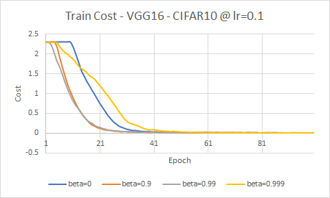by this definitions new update rule based on $V$ is as follow: Equation 22: $\Delta W_t=-l V_t$ below figure shows the effect of different values of $\beta$ on loss reduction:

after some experiments involving changing value of $\beta$, we find out the optimal value for $\beta$ in most cases is $0.9$ although may be in some special cases tuning is required. while moving average helped gravity in initial speed but still we can see some delay. for solving this issue we propose an alternative value of $\beta$. any specific value of $\beta$ averages over a number of previous data. actually we can find number of data included in average by below equation: Equation 23: $number \ of \ averaged \ data \approx \frac{1}{1-\beta}$ but at the first epochs there is not enough data to be averaged and also at the beginning of the training, which $t$ is small and $V_0=0$, the value value of equation 21 will be very small. there is a solution known as bias correction which modifies $V_t$ as follow: Equation 24: $V_{t}=\frac{\beta V_{t-1}+(1-\beta)\zeta}{1-\beta^t}$ the logic behind equation 24 can be explained as follow: by increasing the value of $t$ the denominator approach to $1$ and equations 24 and 21will output almost same result. but at the beginning of the training the value of $1-\beta^t$ is small and dividing equation 21 to this small value increase total outcome. we tried to use bias correction but at large values of $\beta$ (closer to 1) we encounter overflow in our code therefore we tried to solve the problem of equation 21 at initial steps with different approach. we propose an alternative to beta as follow: Equation 25: $\hat{\beta} = \frac{\beta t+1}{t+2}$ value of $\hat{\beta}$ in equation 25 at large $t$ will tends to $\beta$ but at smaller values it will correct the value of $\beta$. lets drive the equation 25. by choosing any value of $\beta$ we will average almost over $\frac{1}{1-\beta}$ data. let say we want to use a variable value of $\beta$ which increase over time and tends to $1$, therefore always average over all data, we call this variable $\hat{\beta}$. for averaging over all data at each step we want to the amount of data that we average on be t+2 (because at $t=0$ there is 2 data $V_0$ and $V_1$). then we can write: $\frac{1}{1-\hat{\beta}}=t+2 \Rightarrow \hat{\beta}=\frac{t+1}{t+2}$ at $t=0$ the value of $\hat{\beta}$ is 0.5 which will average over 2 data ($V_0$ and $V_1$). by increasing value of $t$ the value of $\hat{\beta}$ tends to $1$ which will average over all data. below table show the value of $\hat{\beta}$ for different values of $t$: as you can see at each step the amount of data that we average on is equal to total available data. for averaging over $\frac{1}{1-\beta}$ we modify above equation as $\hat{\beta} = \frac{\beta t+1}{t+2}$ which is equation 25. now by increasing the value of $t$ the value of $\hat{\beta}$ tends to $\beta$. below figure demonstrate behavior of $\hat{\beta}$ for different values of $\beta$.

in addition to modifying $\beta$ in equation 21 we came out with another solution for increasing the speed of optimizer at early steps by using non-zero initial $V$. instead of zero we initialized $V$ with random numbers with normal distribution with mean $\mu$ as 0 and standard deviation as follow: Equation 26: $\sigma=\frac{\alpha}{l}$ lets look closely at first update step: Equation 27: $\Delta W_0 = -l (0.5 V_0 + 0.5 \zeta_0)$ we can think about this equation as two separated part first part is $\Delta W_{V_0}$ which is due to initial $V$ and second part $\Delta W_{\zeta_0}$ which is due to gradient term. we cannot do anything about gradient term and this part is determined by many different parameters. but we can tweak $\Delta W_{V_0}$for better initial loss reduction speed. 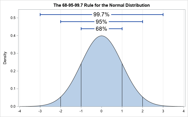first lets define this term as follow: Equation 28: $\Delta W_{V_0} = -0.5 l V_0$ by choosing $V_0=0$ we give total control of optimizer to unknown part of equation 27 which is $\Delta W_{\zeta_0}$. for a normal distributed set of random numbers the 68% of random values are less than standard deviation $\sigma$ and 95% of random number are less than $2\sigma$ and 99.7% of numbers are less than $3\sigma$ there for by choosing $\sigma$ we define the range of initial steps for different parameters. by choosing any $\sigma$ 68% of parameters are $|\Delta W_{V_0}|&lt;\frac{l \sigma}{2}$. we define the numerator of right side of this inequality as a new hyper-parameter called $\alpha$ for controlling value of initial steps: Equation 29: $\alpha = l \sigma$ in fact the equation 26 is same different form of equation 29. by experimenting with different values of $\alpha$ we found $\alpha=0.05$ satisfying for majority of models.

Conclusion

We propose new optimizer for deep learning based on back-propagation from a kinematic point of view perspective. the summary of our algorithm is:

Require: $l$: Learning Rate Recommended Value: 0.1 Require: $\alpha$: Initial Step Size due to $V$ Recommended Value: 0.05 Require: $\beta$: Moving Average Rate $\in [0, 1]$ Recommended Value: 0.9 Require: $t_{max}$: maximum number of update steps

for each parameter: $\mu \gets 0$ $\sigma \gets \frac{\alpha}{l}$ $V_0 \gets{\mathcal {N}}(\mu, \sigma)$

$t \gets 0$ while t<$t_{max}$: $t \gets t+1$ $\hat{\beta} \gets \frac{\beta t +1}{t + 2}$ for each weight matrix $W$: $G \gets \frac{\partial{J}}{\partial{w}}$ gradient of objective function J w.r.t W _ $m \gets \frac{1}{max(abs(G))}$ $\zeta \gets G \oslash (1+(G \oslash m)^2)$ $V t \gets \beta V{t-1} + (1-\beta)\zeta$ $W \gets W - l V_t$ note: $\oslash$ is element wise division also known as Hadamard division

for convenient and we prepared keras implementation of gravity optimizer as follow:

class Gravity(tf.keras.optimizers.Optimizer):
    def __init__(self, learning_rate=0.1, alpha=0.01, beta=0.9, name="Gravity", **kwargs):
        super(Gravity, self).__init__(name, **kwargs)
        self._set_hyper('learning_rate', kwargs.get('lr', learning_rate))
        self._set_hyper('decay', self._initial_decay)
        self._set_hyper('alpha', alpha)
        self._set_hyper('beta', beta)
        self.epsilon = 1e-7
    def _create_slots(self, var_list):
        alpha = self._get_hyper("alpha")
        stddev = alpha/self.learning_rate
        initializer = tf.keras.initializers.RandomNormal(mean=0.0, stddev=stddev, seed=None)
        # initializer = 'zeros'
        for var in var_list:
            self.add_slot(var, "velocity", initializer=initializer)

    @tf.function
    def _resource_apply_dense(self, grad, var):
        # Get Data
        var_dtype = var.dtype.base_dtype
        lr_t = self._decayed_lr(var_dtype) # handle learning rate decay
        beta_hat = self._get_hyper("beta", var_dtype)
        t = tf.cast(self.iterations, float)
        beta = (beta_hat*t + 1 )/(t + 2)
        velocity = self.get_slot(var, "velocity")

        # Calculations
        max_step_grad = 1/tf.math.reduce_max(tf.math.abs(grad))
        gradient_term = grad / (1 + (grad/max_step_grad)**2)

        # update variables
        updated_velocity = velocity.assign(beta*velocity + (1-beta)*gradient_term) 
        updated_var = var.assign(var - lr_t*updated_velocity)       
        
        # updates = [updated_var, updated_velocity]
        # return tf.group(*updates)
    def _resource_apply_sparse(self, grad, var):
        raise NotImplementedError
    def get_config(self):
        config = super(Gravity, self).get_config()
        config.update({
            'learning_rate': self._serialize_hyperparameter('learning_rate'),
            'decay': self._serialize_hyperparameter('decay'),
            'alpha': self._serialize_hyperparameter('alpha'),
            'beta': self._serialize_hyperparameter('beta'),
            'epsilon': self.epsilon,
        })
        return config