Experimental: CTM Concurrently Coupled with GEOS AGCM using NUOPC
This is the GEOS AGCM coupled to the GEOS CTM coupled using a NUOPC wrapper and running concurrently.
Operationally, the GEOSctm is run offline using data files produced by the model run. This creates a lag-time between the model run and CTM products. By running concurrently with the model, using separate resources, it is hoped that CTM products can be produced more quickly. Additionally, as the CTM is run at a coarser resolution than the model, fewer resources can be used when performing re-gridding on-the-fly as compared to writing data files to disk, reading them in again, and performing re-gridding. There may also be a benefit of more accurate results that are afforded by using smaller interpolation windows than runnning the CTM conventionally and direct access to fields that were previously derived.
To achieve the goal of running the AGCM and CTM concurrently, a functionality that GEOS' MAPL framework does not provide, a generic NUOPC wrapper was created that allows arbitrary MAPL models to be run as NUOPC components. The wrapper maps the MAPL initialization and run steps onto their NUOPC equivalent, and since both MAPL and NUOPC are built upon ESMF they can directly share their underlying data structures such as fields, grids, and states.
The AGCM and CTM were wrapped as NUOPC model components driven by a NUOPC Driver with one-way coupling from the AGCM to the CTM through a custom NUOPC Mediator component that implements time interpolation. The time interpolation allows fields to be coupled less frequently than every timestep. In this case, the AGCM is advanced for a user-configurable amount of time to create the interpolation end points, the connector from the AGCM to the CTM is run, and then both the CTM and AGCM are free to run independently until the next coupling period while the CTM receives interpolated data from the mediator.
Work started with an idealized passive-tracer experiment that was chosen for its simplicity. The AGCM and CTM are run on the same C48 cubed-sphere grid with the same number of processors with time interpolation provided by the mediator running on the same set of processes as the CTM.
The chemistry configuration was then switched to GOCART with CO and CO2 for a more realistic use-case. This configuration requires considerably more exports from the AGCM compared to the previous passive-tracer experiment.
Current work is underway to provide re-gridding capability that allows the two models to run on different grids and have re-gridding provided by the mediator.
These instructions require using shell tcsh.
The GEOS CTM is a stripped-down version of the full atmospheric model that includes just the chemistry and dynamics portions of the model, along with the CTM itself to organize calls to those components and derive fields from meteorological fields provided by analysis files (e.g. MERRA2). The chemistry model is itself a wrapper around other chemistry models (GOCART, GEOSchem) and can be configured in various ways.
In your .bashrc or .tcshrc or other rc file add a line:
module use -a /discover/swdev/gmao_SIteam/modulefiles-SLES11
Now load the GEOSenv module:
module load GEOSenv
which obtains the latest git, CMake, and manage_externals modules.
The code can be obtained on Github at:
git clone git@github.com:GEOS-ESM/GEOSctm.git
then checkout the correct branch
cd GEOSctm
git checkout feature/online-ctm
To checkout the rest of the model using the mepo tool, you run:
mepo init
mepo clone
Building the coupled model can be done be performing the same steps outlined in the GEOS repository on Github using CMake:
On tcsh:
source @env/g5_modules
On bash:
source @env/g5_modules
Make a build directory for an out-of-source build:
mkdir build
cd build
cmake .. -DBASEDIR=$BASEDIR/Linux -DCMAKE_Fortran_COMPILER=ifort -DCMAKE_INSTALL_PREFIX=../install
To build with debug flags add -DCMAKE_BUILD_TYPE=DEBUG to the CMake command.
Then, build the model:
make -j6 install
The experiment must be copied from a directory on Discover into a local directory of your choice.
To copy a concurrent GCM-CTM experiment use:
cp -r /discover/nobackup/wjamieso/experiments/online-ctm_concurrent <EXP DIR>
To copy a sequential GCM-CTM experiment use:
cp -r /discover/nobackup/wjamieso/experiments/online-ctm_sequential <EXP DIR>
Note that a concurrent experiment will require twice as many processors as a sequential experiment
The run script is in the copied experiment director: gcm-ctm_run.j. In that script you will need to change GEOSDIR install directory.
To run the experiment one can submit the run script with sbatch gcm_ctm_run.j or request an interactive session with at least 12 processors and run the script directly.
Currently only the resolutions: C48 and C90 are fully supported with the nuopc_setup script.
To create a new experiment on Discover you first need to copy the experiment templates to your repository's install bin after building it:
cp -R /discover/nobackup/wjamieso/ctm_online_templates/* /path/to/repository/install/bin/.
You then can run the setup script inside the install bin using:
cd /path/to/repository/install
~wjamieso/bin/nuopc_setup
and then answering the questions the script asks. Note that the experiment directory needs to already exist, and its default value is given by the value of the environment variable EXPERIMENTS.
The script creates an experiment in /path/to/experiment directory/experiment name as based on the answers you provided. To run an experiment you need to create or copy the correct restarts and cap_restart files for the GCM. One can copy an example set of restarts using
cp /discover/nobackup/wjamieso/ctm_online_restarts/restarts/<RESOLUTION>/* <EXP DIR>
where <RESOLUTION> is the resolution you chose for the GCM and <EXP DIR> is the experiment's directory.
Note that the nuopc_setup script can recreate any experiment without the need to answer any questions by using the answers.yaml file it created in the experiment directory. Note that either the experiment name needs to be different and or experiment overwrite needs to be set to true in order to directly create an experiment using the answers.yaml file. To do this copy the templates used to the new model install directory using:
cp -R <EXP DIR>/templates/* /path/to/new repository/install/bin/.
Then one can create an identical setup using:
cd /path/to/new repository/install
~wjamieso/bin/nuopc_setup <EXP DIR>/answers.yaml
CTM options are configured through the CTM_GridComp.rc resource file. In here settings for passive-tracers, convection, and diffusion can be set.
ENABLE_pTracers: With this option set the chemistry component will not be used and the CTM will be initialized with artificial passive tracers. If this option is set to false then the GEOSchemistry component is initialized which can itself use different chemistries such as GOCART or GEOSCHEMchem, etc.
online_ctm: - This should be set to true when the CTM is being provided fields through NUOPC.
GOCART is configured through several resource files located in the experiment/RC directory.
CTM_GEOS_ChemGridComp.rc - Allows choosing how chemistry is configured. For GOCART only ENABLE_PCHEM and ENABLE_GOCART should be set to true. Other chemistry configurations have not been tested yet.
CTM_Chem_Registry.rc - This file specifies which constituents to simulate within GOCART and the number of bins for each constituent.
GEOSCTM.rc - Set the two previous resource files to read (so that the AGCM and CTM can configure their chemistry separately) with the labels GEOS_ChemGridComp_RC_File:, and Chem_Registry_File:
To run the model simply run the gcm-ctm_run.j script interactively or submit it through sbatch. For example:
$ sbatch --account=ACCT_NUM < gcm-ctm_run.j
where ACCT_NUM is a project you have access to.
The AGCM default to 96 processes and the CTM to 24 requiring 120 total. This can be changed by modifying the domain decomposition in AGCM.rc and GEOSCTM.rc and then number of processes the AGCM will run on NUOPC_run_config.txt. With the number of AGCM processes specified the rest will be allocated to the CTM. The CTM runs much more quickly than the AGCM so it can be run on fewer resources.
All fields required by the CTM are provided by the AGCM except emissions which are read from a file by ExtData.
The following fields are exchanged for a GOCART run:
Centered 3d R4 Fields:
-
U;V - eastward, northward wind, m s-1 -
T - air temperature, K -
Q - specific humidity, unitless -
BYNCY - buoyancy of surface parcell, m s-2 -
CNV_QC - grid mean convective condensate, kg kg-1 -
QCTOT - mass fraction of total cloud water - kg kg-1 -
QICN - mass fraction of convective cloud ice water - unitless -
QLCN - mass fraction of convective cloud liquid water - unitless -
CNV_MFD - detraining mass flux - kg m-2 s-1 -
FCLD - cloud fraction for radiation - unitless -
RH2 - relative humidity after moist - unitless -
TH - potential temperature - K
Centered 3d R8 Fields:
-
CX - Eastward accumulated Courant number - unitless -
CY - Northward accumulated Courant number - unitless -
MFX - pressure-weighted accumulated eastward mass flux Pa m^2 s-1 -
MFY - pressure-weighted accumulated northward mass flux Pa m^2 s-1
Edge 3d R4 Fields:
-
ZLE - edge heights - m -
CNV_MFC - cumulative mass flux - kg m-2 s-1 -
KH - scalar diffusivity - m^2 s-1 -
PFI_LSAN - 3d flux of ice nonconvective precipitation - kg m-2 s-1 -
PFL_LSAN - 3d flux of liquid non-convective precipitation - kg m-2 s-1
Edge 3d R8 Fields:
-
PLE0 - pressure at layer edges before dynamics - Pa -
PLE1 - pressure at layer edges after dynamics - Pa
2d R4 Fields:
-
TS - surface skin temperature - K -
PS - surface pressure - Pa -
FRACI - ice covered fraction of tile - unitless -
FRLAKE - fraction of lake - unitless -
LWI - land-water-ice-flag - unitless -
FROCEAN - fraction of ocean - unitless -
ITY - vegetation type - unitless -
LFR - lightning flash rate - km-2 s-1 -
CLDTT - total cloud area fraction - unitless -
CN_PRCP - convective precipitation - kg m-2 s-1 -
DZ - surface layer height - m -
FRLAND - fraction of land - unitless -
FRLANDICE - fraction of land ice - unitless -
GRN - greeness fraction - unitless -
LAI - leaf area index - unitless -
SH - sensible heat flux from turbulence - W m-2 -
SWNDSRF - surface net downward shortwave flux - W m-2 -
TPREC - total precipitation - kg m-2 s-1 -
TSOIL1 - soil temperatures layer 1 - K -
U10M - 10 meter eastward wind - m s-1 -
U10N - equivalent neutral 10 meter eastward wind - m s-1 -
USTAR - surface velocity scale - m s-1 -
V10M - 10 meter northward wind - m s-1 -
V10N equivalent neutral 10 meter northward wind - m s-1 -
WET1 - surface soil wetness - unitless -
Z0H - surface roughness for heat - m -
ZPBL - planetary boundary layer height - m -
TROPP_BLEND - tropopause pressure based on blended estimate - Pa -
TA - surface air temperature - K
A PTracer experiment only needs a subset of the imports required by a full chemistry run.
-
CX, CY -
MFX, MFY -
PLE0, PLE1 -
PS -
Q -
TH -
LWI -
ZLE
The wrapper and coupled model were tested in several stages.
A simple idealized passive-tracer configuration was initially used with coupling from the model to the CTM at every timestep due its simplicity and low number of coupled fields. Conservation of tracer mass and visual inspection of the tracers compared to a conventional CTM run were used to compare. Bitwise identical results are not possible due to differences in using data directly from the model and interpolated data from disk.
Then, the mediator was implemented and the interpolation was tested by setting the interpolation interval equal to the timestep so that the interpolation weights were 1.0 and 0.0, a copy. The fields output from the mediator were found to be bitwise identical to directly copying the fields.
The interpolator was then tested with a longer coupling period with artifical data and was verified to be correct (i.e. the starting field was set to 0 and end field was set to 1 with 4 interpolations and the output was 0.0, 0.25, 0.5, 0.75).
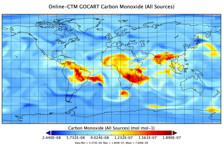
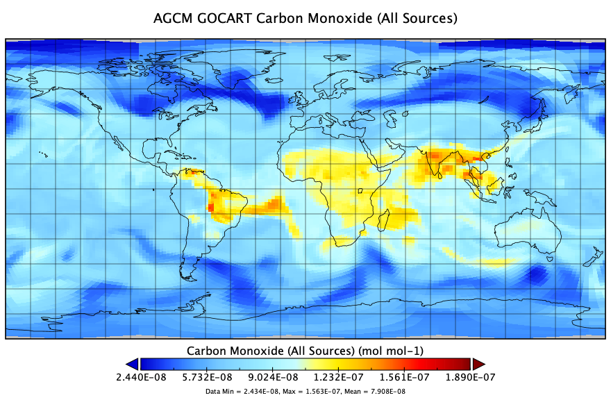
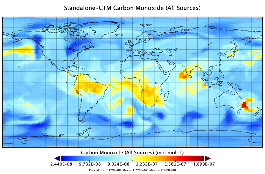
GOCART was verified and validated by comparing it to a CTM run and to an AGCM chemistry run with the same chemistry configurations. In GOCART CO with 10 bins and CO2 with 1 bin were enabled
An experiment was run with three different configurations all running CO in GOCART: One with the online CTM, one with the internal AGCM chemistry, and one with the standalone CTM. The models were run for one month in October 2014. The online CTM behaved in a reasonable manner; the model didn't blow up and the fields look reasonable in their general structure compared to the AGCM. Though the concentrations are lower, but this may be due to the differences in the way chemistry and dynamics are run in the full model compared to the simplified CTM model.
A series of benchmarks were performed to measure the effect of running the CTM concurrently with the AGCM. First, a base case was run to measure the AGCM without the CTM. Then, the CTM was run concurrently on varying numbers of processors with different time-interpolation interval at C360: from 6 hours, down to exchanging the fields every timestep, while the AGCM was run on a constant 1536 processors at C720 resolution.
Depending on the number of processors running the CTM resulted in a slowdown of anywhere from ~2% with a 6-hr exchange of fields and 384 processors, up to ~20% exchanging fields every timestep on 96 processors.
