Home

Probe Particle Scanning Tunnelling Microscopy (PPSTM) simulation package:

Overview:

A Python3/C++ software package for simulating couple of Scanning Tunnelling Microscopy - STM techniques based on results of electronic-structure computations (Density Functional Theory - DFT) using local basis set (LCAO). New users should have some experience with DFT computations and some overview of STM (e.g. 2nd chapter here)

Compilation:

Written in Python 3 (operating language)/C++ (heavy machinery, via C_types) or optionally Python/OpenCL for run on graphics card. The later option works only for one example and is under (sleeping) development.

2 OS compilations working and tested:

Linux -- compilation should work automatically with usage of g++ compiler
MAC -- OS set automatically, g++-9 set as default; adapt your makefile in cpp/ folder and/or your (MCC) compiler using this.
Windows not tested, please contact us, if you run into problems.

Serial or OpenMP parallelisation:

Decided automatically depending on the system OMP_NUM_THREADS variable -- if it is 1, or not set, then serial ; otherwise OpenMP.
Code is compiled each time it is run,

Makefile is in cpp/ folder.

GUI for more user friendly experience:

In order to run the interface, clone the repository using: > git clone https://github.com/Probe-Particle/PPSTM.git
And follow the instructions from the full descrtipion of GUI

Software requirements

Python 3.7 with following packages:Numpy, matplotlib and PyQt5(for GUI)
GCC 9.3 or higher, alternatively clang 10.0 or higher. BEWARE of problems with MAC default gcc compiler - look here for possible solutions.

Developers:

Mainly developed at: Nanosurf Group, Institute of Physics of the Czech Academy of Sciences, Czech Republic and SIN group, Aalto University, Finland; with help from: Nanotech@surface Laboratory, EMPA, Switzerland. Contacts

Literature:

The structure of the code and how it works is explained mainly in the literature:

Main principle of STM and dI/dV calculations: Ondrej Krejčí, Prokop Hapala, Martin Ondráček, and Pavel Jelínek, Principles and simulations of high-resolution STM imaging with a flexible tip apex, Phys. Rev. B 95, 045407 – Published 6 January 2017 https://journals.aps.org/prb/abstract/10.1103/PhysRevB.95.045407
Main principle of IETS calculations and usage of d-sample orbitals: Bruno de la Torre, Martin Švec, Giuseppe Foti, Ondřej Krejčí, Prokop Hapala, Aran Garcia-Lekue, Thomas Frederiksen, Radek Zbořil, Andres Arnau, Héctor Vázquez, and Pavel Jelínek, Submolecular Resolution by Variation of the Inelastic Electron Tunneling Spectroscopy Amplitude and its Relation to the AFM/STM Signal, Phys. Rev. Lett. 119, 166001 – Published 16 October 2017 https://journals.aps.org/prl/abstract/10.1103/PhysRevLett.119.166001
More detailed description in a thesis of Ondřej Krejčí: DFT simulations of interaction of organic molecules with oriented surfaces , chapters 4 and 8. These chapters also contain the original papers above.
For simulations of images obtained with flexible tip apexes please read about the Probe Particle Model (PP-AFM), whose calculations are necessary for these types of simulations: https://github.com/ProkopHapala/ProbeParticleModel/wiki and https://nanosurf.fzu.cz/wiki/doku.php?id=probe_particle_model (To be updated later)

Preparing Inputs with DFT codes:

Suggestion: It is better to run a geometry optimisation in a first run and then create the inputs for STM calculations, and possibly AFM pre-calculation, in a separate single-point calculation using the optimised geometry.

How to create the input files for the STM part of the Probe Particle is written here. You can also look to the ASE useful scripts for writing/creation the input geometry files.

This is also true for calculations with the 'fixed tip'.

For the runs with 'flexible tip apices' and for storing in xsf and npy format you must have PPAFM(>=0.2.0a3) installed. You can easily do it by running: pip install ppafm>=0.2.0a3.

For additional pre-calculation for the 'flexible tip' simulation and on the best strategy for the simulations, look here.

PPSTM_simple.py

Overview:

Fully automatic (closed) python script for STM and/or dIdV calculations with stiff single atom or flexible tip-apex for calculations of systems on metallic/semiconductor substrates for sample biases between (-2,+2) volts:

You can copy this script to directory with your (DFT and/or PP-AFM) pre-calculations, set properly ppstm_path to your PPSTM code (DO NOT USE $HOME for the path, still both absolute or relative is working) and you can run the script in the folder. Later you will have a possibility to see what options you used for the calculations.

The first part of the script contains variables that you can change, so the code would do, what you want. There is an brief explanation for each variable at the end of the line in comments. The script should be self-explaining.

All the Voltages are defined with respect to the sample (positive ~ empty states, negative ~ filled states) and the Fermi Level.

DFT codes inputs:

The script can handle DFT inputs pre-calculated from Fireball, CP2K, FHI-AIMS and GPAW (in LCAO mode) codes. How to prepare those inputs is explained here. The script was tested for first three DFT-codes (fell free to test GPAW, but it has known problems for handling d orbitals on the sample and if any Hydrogens are not at the end of contributing atoms).

For CP2K and FHI-AIMS spin-polarized calculations can be handled as well. You can choose 'alpha' = 'up' spin, 'beta' = 'down' spin or 'both' spins contributing to your current.

Types of calculations/scans:

didv - single dI/dV (conductance) calculation at the energy (relative to the Fermi Level) given by V .

USE 'V-scan' instead of 'STM': 'STM' is calculated via rectangular integration = SUM of single dIdV for a single voltages between required voltage and zero. At the end it gives you a data for a single voltage V-scan, on the other hand, is basically calculating all dIdVs between Vmin and Vmax ( Vmin<=0<=Vmax ), then calculates STMs and gives you all of them. You'll therefore have everything between Vmin and Vmax in a single run. If an experimentalist asks you about an image on 1.5 V I would perform V-scan between 0 and 2 V and then looked at the image and compare -- it is possible, that either gap, either the Farmi Level either some state is at wrong energy from your DFT calculations and therefore better STM image can be found on slightly different voltage. (Finally if you want to go over +-2V you have to adjust your cut_min and cut_max accordingly and especially in positive voltage pray, that your God of DFT makes your electronic structure of empty states far above the Fermi Level reasonable.)

For molecules: New feature 'states' : it will make a dI/dV calculations just for such Voltages, that corresponds to the eigen energies (states = ei) of the sample, which are within V <= ei <= Vmax . You do not need to specify those eigen energies by yourself; the script finds them by itself. Beware that still all the states are taken into account for the dI/dV calculations. If you want to use just 1 state, choose very low eta (e.g. 0.0000001).

Periodic Boundary Conditions:

Various Periodic Boundary Conditions (PBC) can be used, but beware:

i) the script cannot use multiple k-points (it can read only Gamma k-point data), therefore that used supercell has to be big enough so the Gamma point will describe the electronic state of your sample properly.

ii) The script do not fold the scanning points into the original cell, therefore you can (sometimes) find the 'ends' of your geometry with 'boundary effects' taking place there. If electronic structure is right (!), those effect cannot penetrate inside into the inner part of the original super cell, but they affect couple of Å nearby the end of geometry.

iii) If electronic structure is OK you can: a) enlarge the amount of multiplied cells and use the inner part only (possible with the PPSTM_simply.py script). Or b) come up with procedure that will fold the positions into the original supercell (not written yet, one of the TODO goals).

Meaning of sample orbitals:

Orbitals of the sample are not directly connected with used LCAO basis-set of your DFT calculations. Even though you can use very big basis set for any element, the PPSTM code uses only valence orbitals. Therefore you can use only sp sample orbitals, if your top-most atoms (those which are contributing to the current) are up to 3rd period of elements (even though i.e. you are using spd basis-set orbitals in Fireball.) Since d orbitals of the sample decays to the vacuum faster, than sp orbitals, they are 'dampened' using constant rescaling of 0.2. (The factor is taken from comparison of FHI-AIMS s and d orbitals in the far away. The rescaling is not ideal, but different DFT codes uses different decays for various elements, therefore we found no other simple general rule within philosophy of this code.) Usage of sp orbitals is 2x faster than spd and more tip-atom orbitals are programmed. You can also investigate the difference between sp and spd via comparing tip_orb = s' dIdV scans for a single height in your calculations.

Advanced features:

cut_atoms option can be use for (considerably) speeding up the calculations (,especially for thick slabs and high pbc options). In most cases you can cut-out all the atoms that are 3 Å bellow the top-most (current-important) atom. (By current important, we mean anything that has considerable states on it. I.e. Hydrogens on the flat organic structures has probably much lower contributions than C atoms, then the C atoms counts). Or sometimes hydrocarbons on silicon can has much lower contributions than Si adatoms, then the Si adatoms counts.)

If you have high-electro negativity differences in between atoms contributing to the current always check Hartree potential above these atoms. If big changes of the potential above your top-most atoms appear, try to estimate lower_atoms and_lower_coefs_ (rescaling for highly electro-negative atoms). E.g. for O in carbonyl group of TOAT molecule, the oxygens the lower_coefs were set to 0.5 ( PRB 95, 045407 (2017) ).

Outputs:

Outputs can be in:

grayscale png images -- 2D for each height.
WSxM xyz files -- 2D for each height.
3D XSF files with full stack of data.
3D machine readable npy files with full stack of data.

Outputs can be for different heights, voltages, scanning techniques (STM or dIdV) and tip-atom orbitals:

Tip model and its orbitals:

Tip-atom orbitals are: s, px and py, pz, dz2, dxz and dyz. The two last options works only for sp orbitals of the sample, while the first three are working with both sp and spd orbitals of the sample.

s tip-atom orbital works almost as Tersoff-Hamann theory (PRL 50, 1998 (1983) ) -- it goes beyond this theory, since it takes into account interference effects (as e.g. in ACS Nano 9 (9), pp 9180–9187 (2015) ).

We do not calculate the current for any DFT calculated tip-model. We rather opt for calculations with different tip-atom orbitals and comparison with experiment. For calculations with CO-tip which can be anything between s and pxy tip-atom orbital, depending on sample-bias, tip-base element and structure (from PRL 107, 086101 (2011) -- 50/50 s/pxy -- to PRB 95, 045407 (2017) -- 100% pxy tip) you can try some options like 'spxy' (50/50), 'CO' (13/87 -- PRL 119, 166001 (2017) ), '10spxy' (10/90), '5spxy' (5/95), but better is to calculate s and pxy in two separated runs and save it as npy or xsf. Then you can use SUM_Orb_Contrib.py script to print you any configurations between s and pxy tip-atom orbitals. This is possible, since contributions from different tip-atom orbitals can be simply summed-up.

All the 'fixed' scans are constant-height scans. Those should be done ~ 4 - 6 Å above the highest atom of the sample. To run a single-height scan use: [zmin, zmax>zmax+dz, dz]. For the constant-current scans there is no inner procedure. You can try to run scan for at least 2 Å heights with dz between 0.1 and 0.2, save it as xsf and plot it in VESTA or some similar software. But before you do this try to run a single constant-height scan if your simulations are similar to the experiment. Unless there is some crazy behavior with contrast reverse depending on height, there is no probable way that constant-current simulation would differ a lot from the constant-height one. Also, since I or dIdV ~ Exp(-beta z) you can try to plot the images in a log-scale (Not programmed in PPSTM_simple.py, you can use WSXM for that) to emulate the constant-current scan.

Atoms model plotting:

You can plot the position of atoms into the png figures and into the xsf files, if you have geometry, which you want to plot in an input_plot.xyz file. It can be 'bas' geometry, or it can be 'xyz' geometry with a single empty line bellow the amount of atoms in the file.

GUI for PPSTM code

USAGE

After cloning the repository and compilation:

Go to PPSTM directory
run > python GUI.py

Following interface should appear:

EXAMPLE

In the PPSTM/tests/ directory you can find folders with testing data e.g.4N-coronene. Inside the test folder you will find the already saved GUI options for this test: 4nCoroneneOpt.txt

Now, having GUI in front of you, click Load options, go to the test's directory and choose .txt file with options. Everything is pre-set and should run without bugs
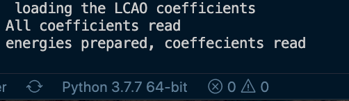
After loading the options, click Import button. Wait for the terminal to say energies prepared, coefficients read
Now click Run

You've successfully run the simulation and plotted the image.

Below you will find more detailed description of each GUI section with the instructions.

INPUT PART

Give requiered input parameters. All the fields in this section are necessary.

codes ~ You can choose form Fireball, FHI-AIMS, CP2K and GPAW
sample orbital ~ either sp or spd
spin ~ none for spin-polarized calculations; up, down or both for spin-polarized calculations
pbc ~ Affects boundary condition. The code is non-periodic from the nature of its design: 00 - calculates current from the original cell only - can be used for a single molecule, or if we want small part of big system; 11 calculated the nature from 3x3 super-cell centred around the original cell; 22 calculated the nature from 3x3 super-cell centred around the original cell - needed if the original cell is very small and we want to calculate big image.
lvs ~ 2D lattice vectors, works as 2D array or a file e.g. input.lvs
Give Input files path which is a path to your directory with necessary data: DFT pre-calculated eigen-energies and eigen-vectors and geometry
Give the name of geometry file, together with extension e.g. input.xyz.
Give CP2K/GPAW ~ name used in CP2K or GPAW calculations
cut_at ~ number of atoms that contribute to the tunneling (-1 = all atoms)
lower_atoms ~ works as 1D array of integers; [] = None means that no atoms has lowered hopping; Be aware that python numbering occurs here: [0] -- means lowering of the 1st atom; [0,1,2,3] -- lowering of 1st 4 atoms
lower_coefs ~ works as 1D array of floats; [] = None means that no lowering of the hoppings; [0.5] -- lowering of the 1st atom hopping to 0.5; [0.5,0.5,0.5,0.5] -- lowering of 1st 4 atoms to 0.5

Now click Import ~ without importing, you won't be able to run the program.

If everything went correct, last line of the output should print: energies prepared, coeffecients read

RUNNING OPTIONS PART

1st line: format, K, Q

Those parameters are used for relaxed scan (i.e. tip type = relaxed) for which you need to have pre-calculated tip-positions in Kx.xxQx.xx/PPpos_*.xsf or .npy files.

Format ~ choose if you need tip-positions as .xsf or .npy files

K ~ radial stiffness

Q ~ charge

Both Q and K are used for PPAFM calculations.
Following 3 lines of parameters are necessary for creating rectangular cuboid grid. 0, 0, 0 is the beginning of the eucleid system. The height of the scan should be about 4-6 Å above the heighest atom of your system
Next 3 lines consist of parameters for the simulation

Scan type ~ there are 3 options: didv, states and v-scan. The default v-scan is preferred, since it allows you to see all didv and STM maps for <V,0> interval. states are useful for molecular systems - gives all dIdV maps for at energies of all eigenstates in between Vmin and Vmax . didv calculates a single dIdV map at the energy of V.

Eta ~ Width of the Lorentzian function for energy smearing. Deppending on system it can reach various values: for single molecular orbital very low number – 1e-6 eV; For standard slabs – 0.05-0.1 eV; For low layered or small slabs – 0.3-0.5 eV

WF_decay ~ Describes how the Workfunction (barrier and therefore tunneling decay) is changing with increasing/decreasing voltage for each dI/dV step; 1.0 – the change of the tunneling decay scales with the voltage (at V=1.0 is WF=4.0 eV); 0.0 – no change with the voltage

V(min), Vmax ~ aplied sample bias = (energy vs. the Fermi Level in eV)

dv ~ It's a step between single dIdV calculations in case of V-scan. dV~eta

tip orb s ~ contribution to the tunneling to/from s orbital on the PP

tip orb pxy ~ contribution to the tunneling to/from non-tilting px and py orbitals on the PP (px contribution = py contribution = tip orb pxy /2)

OMP_NUM_THREADS ~ number of cpu cores for OMP paralelization: ncpu = 1 -- serial compilation & calculations; if ncpu > 1, then OMP paralel recompilation is used and C++ calculations are running on more cores

Tip type ~ fixed/relaxed, corresponds to fixed or relaxed scan
Now click Run

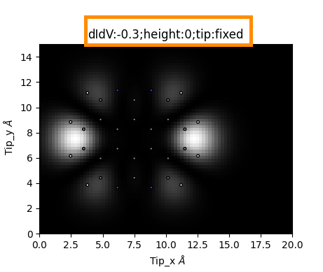
The main part of PPSTM code will run and the program will plot the first image. (By default it is: didv, height:0 , voltage: 0. You can change that before clicking Run if you want)

PLOTTING PART

You can now change the plotted map with the following steps:

choose map type: STM / didv

STM is only available if the scan type was chosen to be v-scan
choose height and voltage index

Voltage index corresponds to different voltages if scan type was chosen to be v-scan or states
Now click Show

You will see that the title of the plot changed to display your chosen map parameters

You can now save the image or the calculated data with the save image and save data buttons respectively:

After clicking the button, in both cases the saving file window will pop up
You can save the image as .png file
In order to save the data, you can choose .xsf, .npy or .xyz extension for it
By default, in both cases the name of the saved file consists of data such as: map type, tip type, WF value, eta value, height and voltage index

In order to save your chosen parameters (from both input part and running options part) you can click save options button

The options will be saved as .txt file with each parameter listed on a new line. You can write your comments into this file by making a new line and beginning a comment with #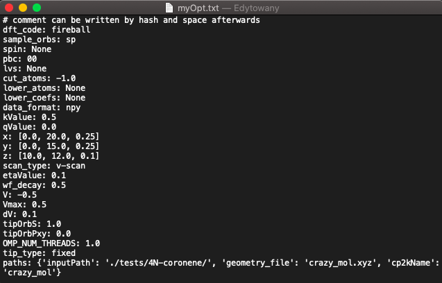

Load options button lets you load those saved options back into the GUI. After clicking it, the file browser will pop up. You just need to select the file with your saved options and click enter.

RELAXED SCAN

In order to run relaxed scan you need to have installed PPAFM code with pip install ppafm>=0.2.0a3.

ADVANCED OPTIONS

If you require to change other parameters, you can inspect them inside pyPPSTM/guiMethods.py

Functions inside guiMethods.py:

imported() ~ code inside this function runs when you click import button
newPPSTM_simple() ~ this corresponds to button Run and it calculates the main results

Scripting and Development:

Except for the 'closed' PPSTM_simple.py script and GUI, there is always a possibility for your own scripting. (But beware of necessary debugging):

You can look into a Si 7x7 example script to see how to calculated STM and dI/dV images with 'fixed tip'
An example how to run 'flexible tip' simulations with whole PP-AFM pre-calculations and the PP-STM calculations is in tests/4N-coronene/run_test.sh. The script how to calculate the PP-dI/dV is in dIdV_test_4N-coronene.py and dIdV_test_4N-coronene.py_cp2k . For this kind of calculations a linking with PP-AFM code needs to be done: To read the positions of the relaxing PP the 'ppafm.io' are important. PP-AFM linking is also needed once you want to plot df together with STM.
To understand the input parameters of inner dIdV and STM calculating procedure, look into input parameters of the running procedures.
To understand how the input files (from DFT codes) are read, look into reading parameters.

Examples and Tests :

Example of STM with rigid tip Si (111) 7×7 reconstruction: Si_7x7
Example of dI/dV scans above spin-polarized CuPc molecule with rigid tip: CuPc
Example of PPSTM simulations with flexible CO tip: 4N-coronene
Example of PP-IETS simulation with flexible CO tip: FePc_Au

TODO :

(but I will probably not have time to do it any time soon. Please send me a message if something would be interesting for you, I can try to speed it up.)