Vibrations

VIBRATIONS ANALISYS

1. INTERFACE

DroneCAN doesn't provide an easy way to define a new message for our purposes, so let's use the existed, but unused in real applications ahrs.RawIMU message.

The following fields should be used as they are designed:

• timestamp is always 0 because global network-synchronized time is not supported yet,
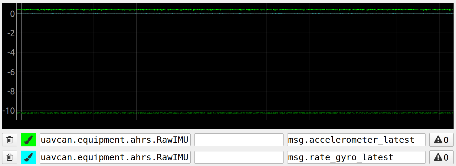
• rate_gyro_latest is the latest gyro measurement,
• accelerometer_latest is the latest accel measurement.

Let's use override the meaning of these fields:

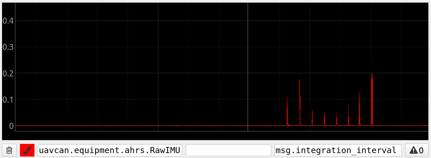
• integration_interval is equal to publishing period in seconds the accel vibration metrics calculated as in PX4,
• rate_gyro_integral is [the dominant frequency, the magnitude of the dominant frequency, 0],
• accelerometer_integral is [the dominant frequency, the magnitude of the dominant frequency, 0].

This message can be used for logging purposes, and we can easily create plots in gui_tool when debugging.

The publishing frequency should be defined by a parameter imu.pub_rate from 0 to 400.

2. PARAMETERS

#	Param	Values	Meaning
1	imu.mode	[0; 4]	Choose the mode of the module 0 - disable the module, do not consume cpu time at all, supress all module related warnings 1 - enable the module and simple RawImu publishing 2 - add vibrations level estimation 3 - run FFT based on accel data 4 - run FFT based on gyro data By default, the imu module should is disabled. No matter what is the value of this parameter, a module should try to initialize mpu9250 at the initialization step.
2	imu.pub_frequency	[0; 400]	This parameter limits the publishing rate (it doesn't affect on the measurement or FFT algorithm). 0 - disable the RawImu publishing, [1;400] - enable RawImu publishing with the given rate. By default, let's publish with 1 Hz by default.

3. USE CASES

1. Raw IMU measurement

The simplest thing is to use a raw imu measurements.

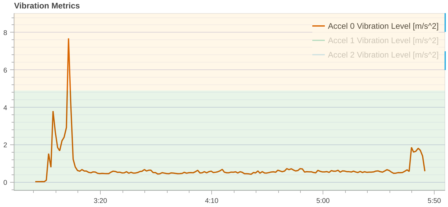
2. Vibrations level measurement

Vibrations metric is calculated as norm of difference beetween norm of measurements processed in moving average filter.

How it is implemented in PX4	How it can be analysed with gui_tool

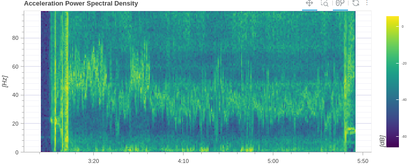
3. Dominant frequency and magnitude measurement

The dominant frequency and the magnitude are calculated with FFT algorithm.

PX4 flight review provides Acceleration Power Spectral Density	We provide only a dominant frequency and a magnitude
	...

in process

4. FFT IMPLEMENTATION DETAILS

Constants

Requirements:

• ICE rotation speed is usually less than: 12000 RPM (200 Hz),
• Motor rotation speed is usually less than 6000 RPM (100 Hz).

So, MPU9250 should measure accelerometer data with 400 Hz rate to capture all frequencies.

So, we have the following constants:

constexpr size_t NUMBER_OF_SAMPLES = 400;

Step 1. Collecting samples

Each sample is a magnitude calculated as:

std::array<float, 3> raw_accel_sample = {{...}};
float magnitude = std::sqrt(std::pow(raw_accel_sample[0], 2) + std::pow(raw_accel_sample[1], 2) + std::pow(raw_accel_sample[2], 2));

Once we have 400 samples, we then handle the following buffer:

std::array<float, NUMBER_OF_SAMPLES> accel_magnitudes;

Step 2. Applying Windowing

Before performing the Fast Fourier Transform (FFT) on the accelerometer data, we apply a Hanning window to reduce spectral leakage. This helps improve the accuracy of the frequency domain representation by tapering the data at the edges, thereby smoothing transitions and reducing the impact of discontinuities between the start and end of the sampled data.

The Hanning window is a type of cosine window and is defined as:

$$ w(n) = 0.5 \times \left( 1 - \cos\left( \frac{2\pi n}{N-1} \right) \right) $$

Where:

• w(n) is the window value at index n.
• N is the total number of samples in the data buffer.
• n is the index of the current sample, ranging from 0 to N-1.
• pi is the mathematical constant (approximately 3.14159).

In result we have a windowed buffer.

std::array<float, NUMBER_OF_SAMPLES> windowed_buffer;

Alternatives. Instead of Hanning window we can sconsider:

• Rectangular (No Windowing). Though it has Poor frequency resolution due to spectral leakage.
• Hann Window has similar to Hamming, but it has slightly worse frequency resolution than Hamming.
• Blackman Window has better leakage reduction but at the cost of lower frequency resolution and higher computational complexity.

Step 3. Applying FFT

The FFT converts the time-domain signal into the frequency domain.

Step 4. Finding peaks

5. REFERENCE

• STM32: CMSIS-DSP
• Ubuntu: fftw3