Pure Pursuit
Adaptive pure pursuit is a path following algorithm for vehicle navigation. The algorithm follows a path as a human driver would by looking ahead at a path and in the direction, updating the point you are looking at to maintain a lookahead distance from you to the point. This algorithm is useful for autonomous and programming skills to follow a very smooth and fast path to your target, eliminating jerky movements that create inaccuracies in odometry, faster paths, flexibility, and a more robust system that can react to outside forces that can impact a robots autonomous routine.
The adaptive pure pursuit algorithm controls a robot on a curved path, to a selected goal point. The algorithm finds a point, a lookahead distance away from the robot, and pursues that point, continuously updating as the robot follows that path. This algorithm mimics one way a human driver would follow a path, by looking ahead at a consistent distance on the road, and pursuing that point.
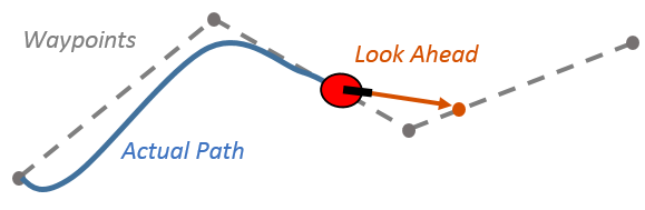
- lookahead distance - The distance that points will be from the robot
- lookahead point - The current point on the path that is one lookahead distance away from the robot
- next point - The point on the path that is next after the current lookahead point.
- goal point - The end point
- current position - The live position of the robot, acquired from the odometry.
- Odometry
- Finding the lookahead point
- Calculate robot movement, and move robot
We have 3 wheel odometry on our current robot that uses 3 perpendicular to the live position of the robot during autonomous operation of the robot. There is more detail about this subject in the 3 Wheel Odometry section of the notebook.
Finding the lookahead point is one of the most challenging parts of pure pursuit. We have accomplished this by handling all of the path mathematics in the path class. To find the appropriate lookahead point we find the intersection of a circle with the same position of the robot and a radius that equals the lookahead distance, and a of the line segment. To find the intersections we a quadratic equation to find if there are any intersections, and calculate the valid results of the calculations.
If the discriminant is more than 0, we know there is a valid answer so we continue, if there is no valid answer we will return nothing. t1 is the first intersection, and t2 is the second intersection.
The result of this is that we have 2 intersections with the line, t1, and t2, although they might not both be on the line segment the largest one that is on the line segment we will return, if none are on the line segment we will return nothing.
To calculate the robot movement we have to get the vector of the lookahead point to the robot’s position to command the robot. To do this we will use our vector utility class to create a vector that equals the lookahead point - current position.
We will put this value through a PID to get a better movement. To do this we will have to scale the vector to match the lookahead distance to make the PID profiles work similar with different lookahead distances. We send this magnitude to a PID to smooth out the values. Before we send the values to the motors, we will multiply them by the curvature of the line to slow down on fast turns. We implemented the most efficient way we could find, normalizing the last movement vector and the current robot movement, to approximate the curvature. We compact this value to the range [0, 1] and multiply that by the PID result, and send that to the motors. The math is below, where l is the the last vector to the lookahead point, v is the current vector to the lookahead point, m is the vector sent to the motor, and c is the vector output of the PID and to the lookahead point.
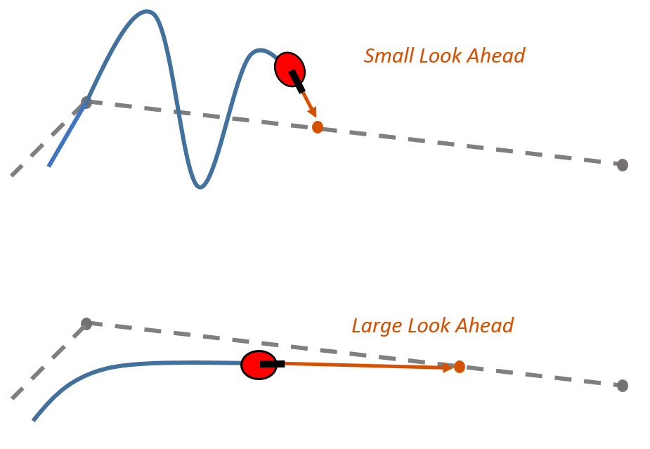
The main variable that you can tune in the pure pursuit algorithm is the lookahead distance. A smaller lookahead distance will regain the path faster, but will have oscillations. A larger lookahead distance will regain path slower in a faster path, and less oscillations. This is illustrated below.
Pure pursuit is a challenging and complex project that we under went. This project did not work at first but after a little debugging we got it working really fast. Our first problem was that it didn't detect the point once it got 1 lookahead distance from the beginning point, after a little debugging, we found that there was a small bug in a dot product in the implementation. Our next problem was if it ever got of the line in sim or on the robot it would go back to the last point and it doesn't make any forward progress. We just used some code to find the closest point to the line.
To test pure pursuit we will run it on complex paths with different objects that it will interact with to test the rigidity of our implementation of the algorithm.
This path runs in a slalom pattern around a few rings to test fast accelerations and motions. We will run a path around rings and if it is able to successfully follow the path without touching any rings, we will record the time in the spreadsheet.
| Image of the path |
|---|
Each of these boxes will be filled with about 10 trials from a spreadsheet.
Each of these boxes will be filled with about 10 trials from a spreadsheet.
Each of these boxes will be filled with about 10 trials from a spreadsheet.
Each of these boxes will be filled with about 10 trials from a spreadsheet.
In tipping point there is the center zone where both teams can interact during autonomous. To test this we will run the robot on a straight path and knock it off path and time how long it takes to get off path.
We will have a 30 in straight path with a 10 inch lookahead distance. We will try to push the robot in a uniform manner to keep consistent test results.
Image of setup
Each of these boxes will be filled with about 10 trials from a spreadsheet.
During autonomous and skills routines we might run into a goal that will perturb our path. We will test what happens when you hit a goal head on, on the side, pushing one from when you start moving, and a control we will do a time trial on a straight line and see how the times differ.
We will have the robot code the same for every time trial with a path that will drive 30 in forward at the start of autonomous. The lookahead value will be 10 inches.
Image of control
Image of head on collision
Image of side collision
Image of push
Each of these boxes will be filled with about 10 trials from a spreadsheet.
Each of these boxes will be filled with about 10 trials from a spreadsheet.
Each of these boxes will be filled with about 10 trials from a spreadsheet.
Each of these boxes will be filled with about 10 trials from a spreadsheet.
Each of these boxes will be filled with about 10 trials from a spreadsheet.
Even though pure pursuit took a lot more time to implement than any other motion algorithm, and it was much more complex, it was worth it in the smooth motions and raw speed, this gives us a huge advantage in autonomous where every second matters when getting the middle goals. Another benefit of using this algorithm is that if we do get off track in autonomous we will be able to regain our path and finish the autonomous and still get points.