Copyright and license

The code and documentation are released under the GPL v2.

Recent changes

A high-level summary of what's changed:

Earth model overhaul — The 3D Earth globe now composites high-resolution local world-map tiles for its surface texture, rendering only the area around the project's location for performance, with a lat/lon grid overlay and elevation-based terrain relief
World and location views — The world map view gained panning, additional zoom levels, and image caching for smoother transitions; the station and EPW file pickers were improved with multi-file support, scrollbars, cancel support, and clearer titles; several weather data sources (EPW/TMY, NAEFS and SWOB) received download upgrades.
Rendering and shadows — Added shadow casting for trees, render preview support, and various shading-quality and viewport-shading improvements.
Editable spinners — Numeric spinner controls throughout the UI can now be edited directly by clicking and typing, with familiar text-entry controls (cursor movement, selection-free editing, Escape to cancel), in addition to the existing drag/click adjustment.
Selection overlays — A dedicated overlay system now draws selection highlights (bounding boxes, edges, pivots) separately from the model geometry, with camera clipping and styling fixes.
Performance improvements — Wide-ranging optimizations across geometry and intersection algorithms, array/memory handling, shading calculations, and the rendering and selection pipelines.
Cross-platform reliability — Replaced a shell/7z dependency with a pure-Java decompression path for better cross-platform support; weather-data API keys are now read from a .env file.
Project structure and internal cleanup — Source files were reorganized under app/src/solarchvision_bim, alongside broad internal refactoring for maintainability.

Installation

Clone using SSH

git clone git@github.com:archmoj/solarchvision_bim.git

or

git clone git@github.com:archmoj/solarchvision_bim.git --depth 1

Clone using HTTPS

git clone https://github.com/archmoj/solarchvision_bim.git

or

git clone https://github.com/archmoj/solarchvision_bim.git --depth 1

Requirements

Processing v4 must be installed, as SOLARCHVISION-BIM is a Processing sketch.

Before running the program

You should adjust the BaseFolder variable inside solarchvision_bim.pde.

String BaseFolder = "/home/solarch/org/solarchvision_bim";

Run using Processing IDE

The solarchvision_bim sketch can be opened in the Processing IDE and executed using the Play button.

Run using command line

To compile and run the solarchvision_bim sketch, adjust <PATH-TO-PROCESSING> in the following command as needed.

Please note that the command must be executed from the parent directory containing the solarchvision_bim folder.

<PATH-TO-PROCESSING>/processing-java --sketch=app/src/solarchvision_bim --run

Download CWEEDS files

For locations in Canada, there is a database called CWEEDS, which includes multi-year climate data under the Engineering Climate Datasets (https://climate.weather.gc.ca/prods_servs/engineering_e.html).

The files for the region of interest can be extracted and placed inside the solarchvision_bim/input/climate/CWEEDS/ folder.

Graphical User Interface

Once loaded the UI would look like this:

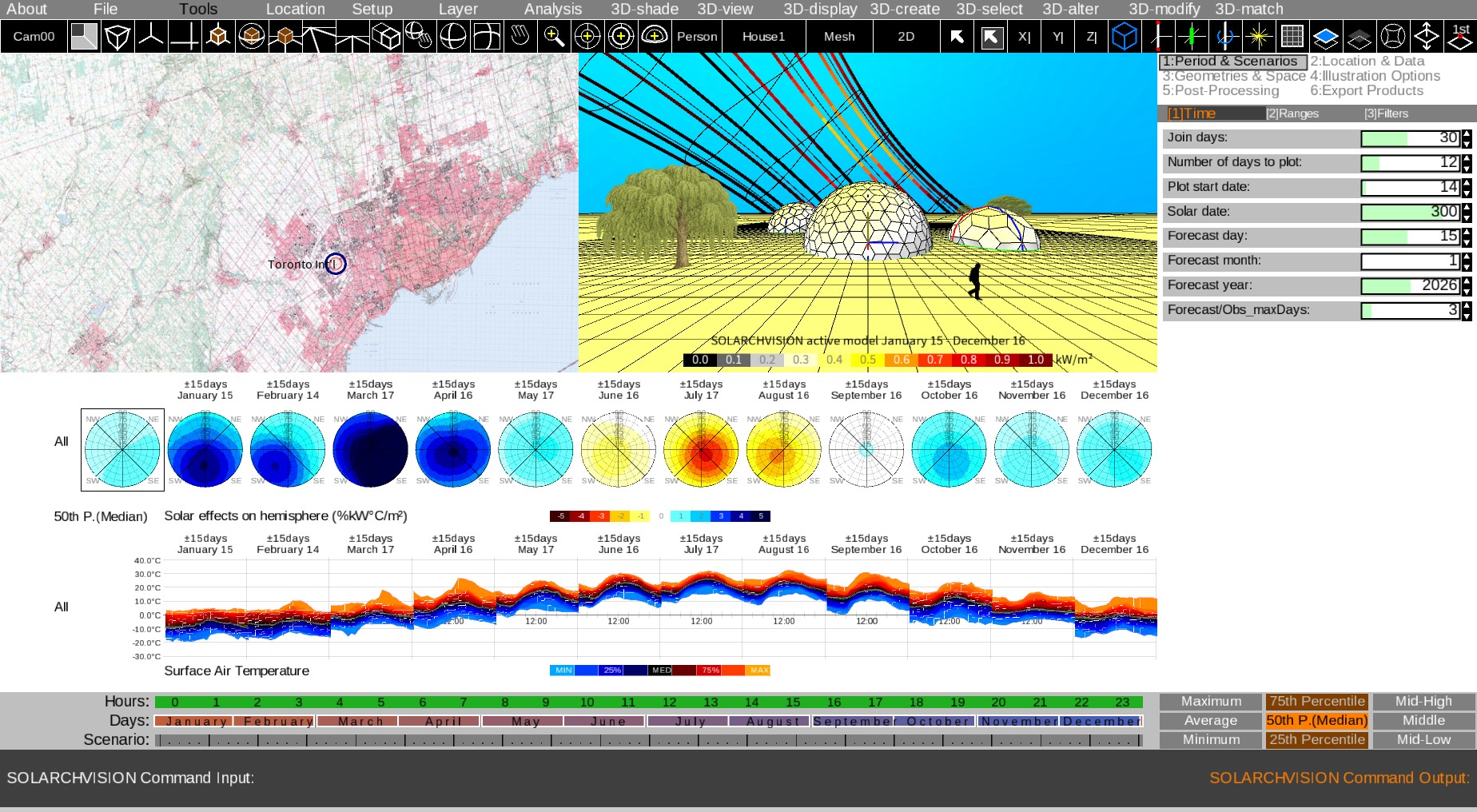
Please note that in above example the Setup | 3D-model 7 option is selected. Also the rendering is set to Shade Global Solar option via 3D-shade menu.

Adding an object to the scene

You can choose a desired object such as Houses, Parametric Surfaces, Box, Cushion, Cylinder, Sphere, Octahedron, Icosahedron, Pyramid, Hyper, Plane, Polygon, Extrude, Surface, Polyline, Point, 1D-Tree, 2D-Tree, Person, and Camera from the 3D-create menu.

After selecting the desired object, you can use either right-click or left-click on a surface in the 3D viewport to add it to the scene:

Right-click adds the object to the land surface.
Left-click adds the object to the surface of existing 3D models.

The default parameters used for creating new objects can be found under Geometries & Space → Create.

Alternatively, you can use the command line to generate new objects. For example, the following command adds a section with width and height of 100 units at a distance of 0.1 units above the origin:

section u=100 v=100 z=0.1

See the Command line section for more information.

Selecting objects

You can use the 3D-select menu to select objects of different types, including Land, 1D, 2D, Group, Face, Vertex, Soft, Solid, Section, Camera, and Polyline.

You can also use the following selection methods:

Pick and Window selection modes to select or deselect objects
Add objects to or remove objects from the current selection
Select all and Deselect all options

It is also possible to convert one selection type to another. For example:

Groups >> Faces selects all faces belonging to the selected group(s)
Faces >> Groups selects all groups associated with the selected face(s)

Altering objects

You can use the 3D-alter menu to modify properties of existing objects.

After selecting a modification option, use the mouse wheel to adjust the object properties interactively.

Modifying objects

The 3D-modify menu provides several modifiers for editing 3D surfaces.

For example, the Insert Corner Openings modifier inserts an opening base parallel to the edges of the selected surface(s).

Matching and aligning objects

You can match and align objects using the 3D-match menu.

Quick layout and 3D setup

The Setup menu provides quick access to predefined:

Time viewport layouts
3D viewport models

You can enlarge the time viewport to expand and view complete layout graphs.

Climatic studies

General studies such as:

Wind pattern (active)
Wind pattern (passive)
Orientation potential (active)
Orientation potential (passive)
Hourly sun position (active)
Hourly sun position (passive)
Annual cycle sun path (active)
Annual cycle sun path (passive)

can be accessed from the Analysis menu. These studies are displayed in the time viewport.

For studies related to the 3D model, such as:

Urban solar potential (active)
Urban solar potential (passive)

you must pre-bake the selected Section or Camera using:

PreBake Viewport, or
Pre-bake Selected Sections

before running the analysis.

Weather layers

Two types of weather layers are defined:

General layers
- Available directly from weather data files
- Missing values may be filled using post-processing techniques
Developed layers
- Not available in the original weather files
- Generated through software post-processing

Location menu

You can use the Location menu to select a project location and download or load weather and geographic data.

By default, the software uses EPW/TMY (Typical Meteorological Year) data.

Additional supported datasets include:

Climate files containing multiple years of data (e.g., CWEEDS)
Ensemble forecast datasets (e.g., NAEFS) for visualization and simulation
Observation datasets (e.g., SWOB records)

Additional features include:

Land Mesh and Land Texture require an API key
Troposphere allows loading WMS forecast data to visualize hourly cloud formations using datasets such as HRDPS (High Resolution Deterministic Prediction System) or GDPS (Global Deterministic Prediction System)

Picking a station on the map

Clicking inside the world viewport assigns the nearest station of the currently active dataset (TMYEPW, CWEEDS, CLMREC, NAEFS, or SWOB) to the project.

Left-clicking also zooms the world viewport in to the most detailed level, to confirm exactly where the click landed. Right-click picks a station the same way but keeps the current zoom level, which is handy for comparing several rough locations across a wider area without the view zooming in on every click.

If one or more stations of that dataset fall within its own search radius of the click, a scrollable picker list appears instead of guessing automatically:

Dataset	Search radius
`TMYEPW`	10 km
`CLMREC`	25 km
`CWEEDS`	50 km
`NAEFS`	50 km
`SWOB`	25 km

While the picker is showing:

Click a row to select that station.
Click anywhere else in the world viewport, or press ESC, to cancel without changing the current selection.
If the list is longer than fits on screen, scroll it with the mouse wheel, drag the scrollbar thumb, or click the scrollbar track to page up/down.

Case bar

The Case Bar is located above the Command Bar. It consists of three range sliders on the left and nine statistical options on the right.

Range Sliders

The range sliders allow users to select the desired:

Hours
Days
Forecast Scenarios (or Years when using long-term input data)

To define a range:

Use left-click to set the start of the range.
Use right-click to set the end of the range.

Statistical Options

The statistical options determine which scenario close to the selected data aggregation is used to run simulations in the viewports. Available options include:

Minimum
Average
Maximum
25th Percentile
50th Percentile (Median)
75th Percentile
Middle
Mid-High
Mid-Low

The first six options compute standard statistical measures based on the selected data range.

The Middle, Mid-High, and Mid-Low options are built-in methods that apply weighted selection criteria to sorted data records.

User interface keyboard shortcuts

When the command bar is disabled (default mode), you can use keyboard shortcuts to perform various tasks.

General

TAB: Enable or disable the command bar
Shift+TAB: Switch between active and passive impact views inside the 3D viewport

Camera and viewport control

` and ~: Cycle backward/forward through the world viewport's zoom levels
+ and -: Zoom in and out in the 3D viewport
Ctrl+, and Ctrl+.: Move the camera closer and farther to the selection
, and .: Move the camera closer and farther
2 and 8: Rotate the camera up and down
4 and 6: Rotate the camera left and right
1 and 3: Move the camera left and right
7 and 9: Move the camera up and down
5: Rotate the camera to look at the current selection (or the origin if nothing is selected)
0: Move the camera closer
/ and *: Move the camera toward and away from the selection
UP, DOWN, LEFT and RIGHT: Rotate the camera around the selection

Selection and scene interaction

DELETE: Delete selected item(s)
Shift+UP, Shift+DOWN: Move/rotate/scale (or change properties of) the selection
c and C: Switch the viewport to available cameras in the scene
ENTER: Rebuild global & vertex solar energy/impact data
SPACE: Move time forward & shade viewport
BACKSPACE: Move time backward & shade viewport

Time, weather, and impact visualization

d and D: Change the impact display day in the 3D viewport
t and T: Change the forecast hour used to display the troposphere

Layout and graph controls

The shortcuts in this section, as well as in "Graph scaling and display options" and "Graph visualization modes" below, act on the time viewport.

Ctrl+UP and Ctrl+DOWN: Change the current weather layer displayed in the hourly graph
Ctrl+LEFT and Ctrl+RIGHT: Change the current impact layer displayed in the daily graph
Ctrl+PAGE_UP and Ctrl+PAGE_DOWN: Switch between the numbered diagram Layouts available from the Setup menu (enlarge the time viewport, i.e. the graph View Layout, to view the full layout)
Ctrl+;: Show or hide the impact summary

Graph scaling and display options

Ctrl+' and Ctrl+": Adjust the vertical scale factor of the hourly time graph
< and >: Increase or decrease the number of joined days (30 days by default for monthly graphs)
( and ): Increase or decrease the number of displayed days
[ and ]: Increase or decrease the horizontal interval used for the probabilities graph
{ and }: Increase or decrease the vertical interval used for the probabilities graph

Graph visualization modes

s and S: Change the sky scenario ("All data", "Sunny", "Partly Cloudy", or "Cloudy")
v and V: Show or hide raw values on the hourly time graph
b and B: Show or hide probabilities on the hourly time graph
n and N: Show or hide statistics on the hourly time graph
m and M: Show or hide sorted values on the hourly time graph

Command line

Use TAB to enable or disable the command line, or click inside/outside the command line area (the dark region at the bottom).

Below is a list of available commands. Both lowercase and uppercase variants are accepted.

CLS: Clears the command line screen
OPEN: Opens a saved project
SAVE.AS: Saves the project with a new name
SAVE: Saves the project
HOLD: Holds the scene
FETCH: Fetches the scene
IMPORT: Imports an OBJ file
EXECUTE: Executes a script file containing multiple SOLARCHVISION commands
EXPORT.OBJ.TIMESERIES: Exports the scene in OBJ format at different hours (multiple files)
EXPORT.OBJ.DATESERIES: Exports the scene in OBJ format at different days (multiple files)
EXPORT.OBJ: Exports the scene in OBJ format
EXPORT.RAD: Exports the scene in Radiance RAD format
EXPORT.SCR: Exports the scene in AutoCAD SCR format
QUIT: Exits the software

Location

LONLAT: Sets the longitude and latitude of the location

LonLat ? ?

Selection and editing

SELECT: Selects various categories

Select all/last/nothing/invert/groups/model2ds/model1ds/vertices/faces/solids/sections/cameras/landpoint

DELETE: Deletes the selection or various categories

Delete all/selection/groups/model2ds/model1ds/vertices/faces/solids/sections/cameras

COPY: Copies the selection

Copy n=? dx=? dy=? dz=? rx=? ry=? rz=?

MOVE: Moves the selection

Move dx=? dy=? dz=?

ROTATE, ROTATEX, ROTATEY, ROTATEZ: Rotates the selection

Rotate[X|Y|Z] r=? x=? y=? z=?

SCALE: Scales the selection

Scale s=? sx=? sy=? sz=? x=? y=? z=?

Object creation

PERSON: Creates a person

Person m=? x=? y=? z=?

TREE2: Creates a 2D tree using vertical and horizontal sections

Tree2 m=? x=? y=? z=? h=?

TREE1: Creates a parametric fractal tree in 3D

Tree1 m=? degree=? seed=? x=? y=? z=? h=? r=? tilt=? twist=? ratio=? base=? Tk=? Lf=?

BOX2P: Creates a box using two corner points

Box2P m=? tes=? lyr=? x1=? y1=? z1=? x2=? y2=? z2=?

BOX: Creates a box using center point, width, length, and height

Box m=? tes=? lyr=? x=? y=? z=? dx=? dy=? dz=? r=?

HOUSE1: Creates a house-like structure with roof folded in all directions

House1 m=? tes=? lyr=? x=? y=? z=? dx=? dy=? dz=? dh=? r=?

HOUSE2: Creates a house-like structure with roof folded in one direction

House2 m=? tes=? lyr=? x=? y=? z=? dx=? dy=? dz=? dh=? r=?

HOUSE3: Creates a house-like structure with roof folded in the second direction

House3 m=? tes=? lyr=? x=? y=? z=? dx=? dy=? dz=? dh=? r=?

CYLINDER: Creates a cylinder

Cylinder m=? tes=? lyr=? x=? y=? z=? dx=? dy=? dz=? deg=? r=?

SPHERE: Creates a sphere

Sphere m=? tes=? lyr=? x=? y=? z=? d=? deg=? r=?

SUPERSPHERE: Creates a supersphere (deforms from cube to star-like object)

SuperSphere m=? tes=? lyr=? x=? y=? z=? dx=? dy=? dz=? px=? py=? pz=? deg=? r=?

CUSHION: Creates a cushion-like object

Cushion m=? tes=? lyr=? x=? y=? z=? dx=? dy=? dz=? deg=? r=?

OCTAHEDRON: Creates an octahedron

Octahedron m=? tes=? lyr=? x=? y=? z=? dx=? dy=? dz=? r=?

ICOSAHEDRON: Creates an icosahedron

Icosahedron m=? tes=? lyr=? x=? y=? z=? d=? r=?

POLYGONMESH: Creates an equilateral polygon mesh

PolygonMesh m=? tes=? lyr=? x=? y=? z=? d=? deg=? r=?

POLYGONHYPER: Creates a hyperbolic surface based on an equilateral polygon

PolygonHyper m=? tes=? lyr=? x=? y=? z=? d=? h=? deg=? r=?

POLYGONEXTRUDE: Creates an extrusion from an equilateral polygon

PolygonExtrude m=? tes=? lyr=? x=? y=? z=? d=? h=? deg=? r=?

Mesh creation

MESH2 to MESH6: Creates meshes using 2 to 6 points

Mesh2 m=? tes=? lyr=? x1=? y1=? z1=? x2=? y2=? z2=?

Viewports

ALLVIEWPORTS: Displays all viewports
ENLARGE3D: Enlarges the 3D viewport

Camera control

Includes commands such as:

PAN, PANX, PANY
LOOKORG, LOOKDIR, LOOKSEL
TRUCKX, TRUCKY, TRUCKZ
ORBIT, ORBITZ, ORBITXY
CAMERAROLL, CAMERAROLLZ, CAMERAROLLXY
TARGETROLL, TARGETROLLZ, TARGETROLLXY
DISTC, DISTZ, DISTXY, DISTP
ZOOM, NORMALZOOM
PERSPECTIVE, ORTHOGRAPHIC

Views

TOP, FRONT, LEFT, RIGHT, BACK, BOTTOM
S.W., S.E., N.E., N.W.

Shading and rendering

SHADE.WIRE: Wireframe view
SHADE.BASE: Base shading
SHADE.WHITE: White shading
SHADE.MATERIALS: Material shading
SHADE.GLOBAL: Global solar values shading
SHADE.REAL: Per-vertex solar values shading
SHADE.SOLID: Solid parameter shading
SHADE.ELEVATION: Elevation shading
SHADE.VIEWPORT: Shades the viewport
PREBAKE.VIEWPORT: Pre-bakes the viewport

Additional resources

BIM6D Presentation

Presentation at Ouranos

TU-Berlin book: Intelligent Design using Solar-Climatic Vision (Energy and Comfort Improvement in Architecture and Urban Planning using SOLARCHVISION)

SOLARCHVISION-BIM — Technical Overview

Overview

SOLARCHVISION-BIM is an open-source Processing/Java-based 3D BIM and environmental simulation platform that integrates building and site geometry with geographic, meteorological, climate, solar, and environmental datasets.

The application combines a custom 3D modeling and geometry engine, interactive CAD-style editing, geospatial visualization, time-dependent solar radiation and shadow analysis, wind-flow visualization, scenario and statistical analysis, and export/persistence workflows in a unified desktop environment.

A central characteristic of the platform is the integration of:

3D / BIM Geometry
       +
Geographic Context
       +
Weather / Climate Data
       +
Time & Scenarios
       +
Environmental Analysis
       +
3D Scientific Visualization

This allows building and urban-environment models to be analyzed using time-dependent environmental and meteorological information rather than being limited to static geometric visualization.

Major Technical Subsystems

1. 3D Modeling and Geometry Engine

SOLARCHVISION-BIM implements its own lightweight geometric modeling system rather than functioning only as a viewer.

Core geometry components include:

Points
Faces
Solids
Groups
Polylines
Materials
1D models
2D models

The geometry system supports vertex and face management, surface normals, tessellation, transformations, rotation, scaling, translation, geometric intersections, surface operations, object grouping, material assignment, visibility, and layer management.

This geometry layer provides the foundation for both visualization and environmental calculations.

2. Interactive CAD-Style Modeling

The application contains dedicated modules for interactive 3D operations, including:

Create
Select
Move
Rotate
Scale
Modify
Clone
Delete
Drop
Edit

Users can create and manipulate objects directly within the 3D environment. The interaction system includes 3D picking, screen-to-world coordinate operations, object and face selection, mouse-based navigation, and CAD-style viewport interaction.

3. Parametric and Procedural Objects

The modeling system supports generated objects and procedural 1D/2D representations.

The procedural vegetation system includes parameters such as species/type, random seed, branching degree, scale, rotation, branch tilt, branch twist, branch ratio, trunk dimensions, and leaf dimensions.

This allows vegetation and environmental context to be represented as computational objects rather than only imported static models.

4. 3D Rendering and Visualization

The application uses Processing's P2D and P3D rendering systems and maintains multiple rendering surfaces for different views.

Major visualization areas include:

3D modeling viewport
Geographic/world viewport
Environmental study viewport
Analytical overlays

The rendering system supports perspective and orthographic views, camera transformations, zooming, rotation, directional views, object-centered navigation, 3D overlays, surface and edge rendering, tessellation control, and analytical visualization.

The rendering architecture includes batching, clipping, caching, and selective geographic rendering to improve interactive performance.

5. Solar Position and Radiation Analysis

Solar analysis is one of the core environmental capabilities.

The system calculates solar position using project geographic coordinates and time information, including latitude, longitude, date, and hour.

Solar calculations incorporate:

Direct radiation
Diffuse radiation
Effective direct radiation
Effective diffuse radiation
Solar direction vectors
Surface geometry
Shading/obstruction effects

A simplified workflow is:

Geographic Location
        ↓
Date / Time
        ↓
Solar Position
        ↓
Weather / Climate Radiation
        ↓
3D Geometry
        ↓
Shadow / Occlusion Analysis
        ↓
Surface Solar Impact
        ↓
Visualization / Statistical Study

6. Surface-Level Solar Analysis

The solar analysis engine can process radiation at a spatially detailed level rather than assigning a single value to an entire building.

The implementation maintains time-dependent arrays for sun direction, unit sun direction, direct radiation, diffuse radiation, effective direct radiation, and effective diffuse radiation.

Solar calculations are combined with geometric surfaces and sub-surface processing to estimate spatially varying environmental impacts.

7. Shadow and Occlusion Analysis

The project contains dedicated shadow-casting and geometric intersection functionality.

Shadow calculations use solar direction, 3D geometry, surface geometry, ray/face intersections, and spatial sections.

This accounts for the effect of surrounding geometry on solar exposure and distinguishes theoretical incoming radiation from radiation affected by the modeled environment.

8. Environmental Impact Fields

The environmental analysis architecture is not limited to object-level results.

The system can calculate impact values at arbitrary 3D positions (x, y, z) and generate spatial fields for environmental quantities.

Impact visualization can include:

Points
Lines
Contours
Raster/image-based representations
3D visualization

This provides a bridge between numerical environmental analysis and spatial scientific visualization.

9. Wind Visualization and Analysis

The project contains a dedicated wind-analysis subsystem.

Components include wind-flow visualization, wind-rose visualization, wind speed, wind direction, and environmental impact calculations.

The system can represent wind as a spatial/vector field around modeled solids and visualize resulting flow or impact patterns in 3D.

10. Weather and Climate Data Integration

SOLARCHVISION-BIM contains dedicated data-ingestion and processing workflows for environmental datasets.

Supported data workflows include:

EPW / TMY
CWEEDS
CLMREC
Ensemble forecast data
Ensemble observed data
Meteorological station data

The architecture separates data acquisition/loading from post-processing and analysis:

Download / Load
      ↓
Data Validation / Processing
      ↓
Post-Processing
      ↓
Environmental Variables
      ↓
Analysis
      ↓
Visualization

11. Ensemble and Scenario Analysis

The project includes dedicated modules for ensemble forecast and observed data.

The analysis engine recognizes ensemble forecast and observation datasets and incorporates them into temporal and statistical study workflows.

The study system supports scenario-oriented analysis, allowing environmental results to be examined across multiple possible weather or climate conditions.

12. Statistical Study Engine

The study engine manages:

Analysis periods
Hours
Days
Scenarios
Filters
Statistical layers
Probability
Percentiles
Sorted data
Normalized data
Trends
Impact summaries

Statistical analysis includes minimum, average, maximum, percentile analysis, probability-based visualization, scenario selection, and statistical filtering.

The system can also identify scenarios that are close to specified daily statistical conditions.

13. Cloud and Atmospheric Scenario Analysis

The study engine can distinguish different atmospheric/cloud conditions, including scenario groups based on total cloud cover.

This provides a mechanism for examining how atmospheric conditions influence solar and environmental results.

14. Geographic and Earth Modeling

The application contains a geographic visualization subsystem centered around an Earth/world model.

Capabilities include:

Latitude/longitude positioning
Geographic projections
World maps
Map tiles
Geographic boundaries
Station locations
Zoom levels
Terrain/land visualization
Project-location-based map rendering

Map imagery can be cached and geographically limited to the relevant project/view region to reduce unnecessary processing and improve performance.

15. Meteorological Station System

The station subsystem connects geographic locations with environmental datasets.

Station information can include:

Station code
City
Province
Country
Elevation
Latitude
Longitude
Time longitude
Dataset filenames

Supported station-related datasets include NAEFS, CWEEDS, TMY/EPW, CLMREC, and observational datasets.

This creates a direct relationship between:

Project Location
      ↓
Meteorological Station
      ↓
Environmental Dataset
      ↓
Environmental Analysis

16. Sun, Moon, Sky, and Atmospheric Visualization

The 3D environment includes dedicated representations of the Sun, Moon, Sky, and Troposphere.

The sun model is connected to solar-position calculations, making the celestial visualization consistent with analysis time and geographic location.

The atmospheric visualization subsystem supports time-dependent imagery and geographically bounded image layers.

17. Time-Dependent Simulation

Time is a fundamental component of the platform.

The application maintains temporal state including year, month, day, hour, day-of-year, and analysis period.

Environmental calculations can therefore be evaluated across:

Hours
Days
Seasons
Annual periods
Forecast periods
Multiple scenarios

18. Multi-Viewport Architecture

The application separates visualization into several functional views.

3D View — modeling, camera navigation, object manipulation, and environmental visualization.

World View — geographic context, map visualization, station locations, and geographic data.

Study View — statistical analysis, environmental results, scenario analysis, and time-series visualization.

19. Command-Line and Scripting System

SOLARCHVISION-BIM includes an internal command-line system.

Commands can be entered interactively and can also be executed from scripts/text files. The command system supports parameterized commands using key/value-style arguments.

This provides an additional automation and reproducibility mechanism alongside the graphical interface.

20. Project Persistence

The application contains project save/load functionality using structured XML data.

Project information can include:

Model geometry
Layers
Materials
Station information
Time state
Study configuration
Analysis settings
Object properties

21. Layer and Material Systems

The layer system provides a common abstraction for environmental and visualization variables.

Layers can include ID, unit, name, descriptions, scale, offset, and display thresholds.

The material system associates materials with geometric faces and supports consistent rendering and object representation.

22. Import and Export

The application provides multiple export workflows, including:

OBJ geometry
Time-series OBJ
Date-series OBJ
RAD
SCR
HTML

The OBJ time/date-series export is useful for transferring time-dependent model states or analytical geometry into external workflows.

Architecture at a Glance

                       SOLARCHVISION-BIM
                              │
        ┌─────────────────────┼─────────────────────┐
        │                     │                     │
   3D/BIM Model         Climate / Weather      Geospatial
        │                     │                     │
   ┌────┼────┐          ┌─────┼─────┐          ┌────┼────┐
   │    │    │          │     │     │          │    │    │
 Points Faces Solids   EPW  CWEEDS Ensemble   Earth Maps Stations
   │    │    │          │     │     │          │    │    │
   └────┼────┘          └─────┼─────┘          └────┼────┘
        │                     │                     │
        └─────────────────────┼─────────────────────┘
                              │
                     Time / Scenario Engine
                              │
                 ┌────────────┼────────────┐
                 │            │            │
               Solar        Shadow        Wind
              Analysis     Analysis     Analysis
                 │            │            │
                 └────────────┼────────────┘
                              │
                     Statistical Studies
                              │
                 ┌────────────┼────────────┐
                 │            │            │
             3D View      Study View    World View
                 │            │            │
                 └────────────┼────────────┘
                              │
                    Export / Persistence

Technical Character

SOLARCHVISION-BIM combines:

3D computer graphics
Computational geometry
BIM / CAD modeling
Scientific computing
Environmental simulation
Solar-energy analysis
Meteorological data processing
Climate-data analysis
GIS/geospatial visualization
Statistical/scenario analysis
Interactive visualization
Data import/export
Scriptable workflows

The most significant architectural characteristic is the integration of geometric modeling and environmental data.

A conventional BIM workflow primarily represents buildings and their relationships. A conventional scientific-visualization workflow primarily represents datasets. SOLARCHVISION-BIM connects the two:

Building / Urban Geometry
          +
Geographic Location
          +
Weather / Climate Data
          +
Time / Scenarios
          ↓
Environmental Simulation
          ↓
Spatial Impacts
          ↓
Interactive 3D Visualization
          ↓
Statistical Study / Export

This makes the platform suitable for environmental and climatic analysis of buildings and urban environments.

Name		Name	Last commit message	Last commit date
.github/workflows		.github/workflows
app/src/solarchvision_bim		app/src/solarchvision_bim
doc/images		doc/images
import		import
input		input
scripts		scripts
test		test
.gitignore		.gitignore
LICENSE.md		LICENSE.md
README.md		README.md
run.sh		run.sh

Latest commit

History

Folders and files

Repository files navigation

Table of contents