A Tensor & Deep Learning framework - It's like PyTorch meets SymPy.
Tensorgrad is an open-source Python package for symbolic tensor manipulation. It performs any simplification described in the Tensor Cookbook (draft) automatically, and can even be used as a machine learning framework.
Install tensorgrad via pip:
uv pip install tensorgrad(Optional) For diagram visualizations (LaTeX/TikZ), install:
apt-get install texlive-luatex texlive-latex-extra texlive-fonts-extra poppler-utilsOn macOS, if you encounter 'algorithm' file not found errors when using PyTorch's torch.compile feature, you'll need to use Homebrew's LLVM compiler:
# Install LLVM if not already installed
brew install llvm

# Run Python with the correct compiler
export CXX=/opt/homebrew/opt/llvm/bin/clang++
python your_script.py
This issue affects scripts using torch.compile (e.g., examples with PyTorch backend). The default macOS clang++ is missing C++ standard library headers needed by PyTorch's compiler.
To run the examples for yourself, use the playground or see this notebook.
examples/mingpt.py is karpathy's
minGPT rebuilt as a tensorgrad program
and trained on his sorting task — with torch.set_grad_enabled(False) at the
top. There is no autograd: every gradient is a symbolic derivative, compiled
together with the loss into one fused program:
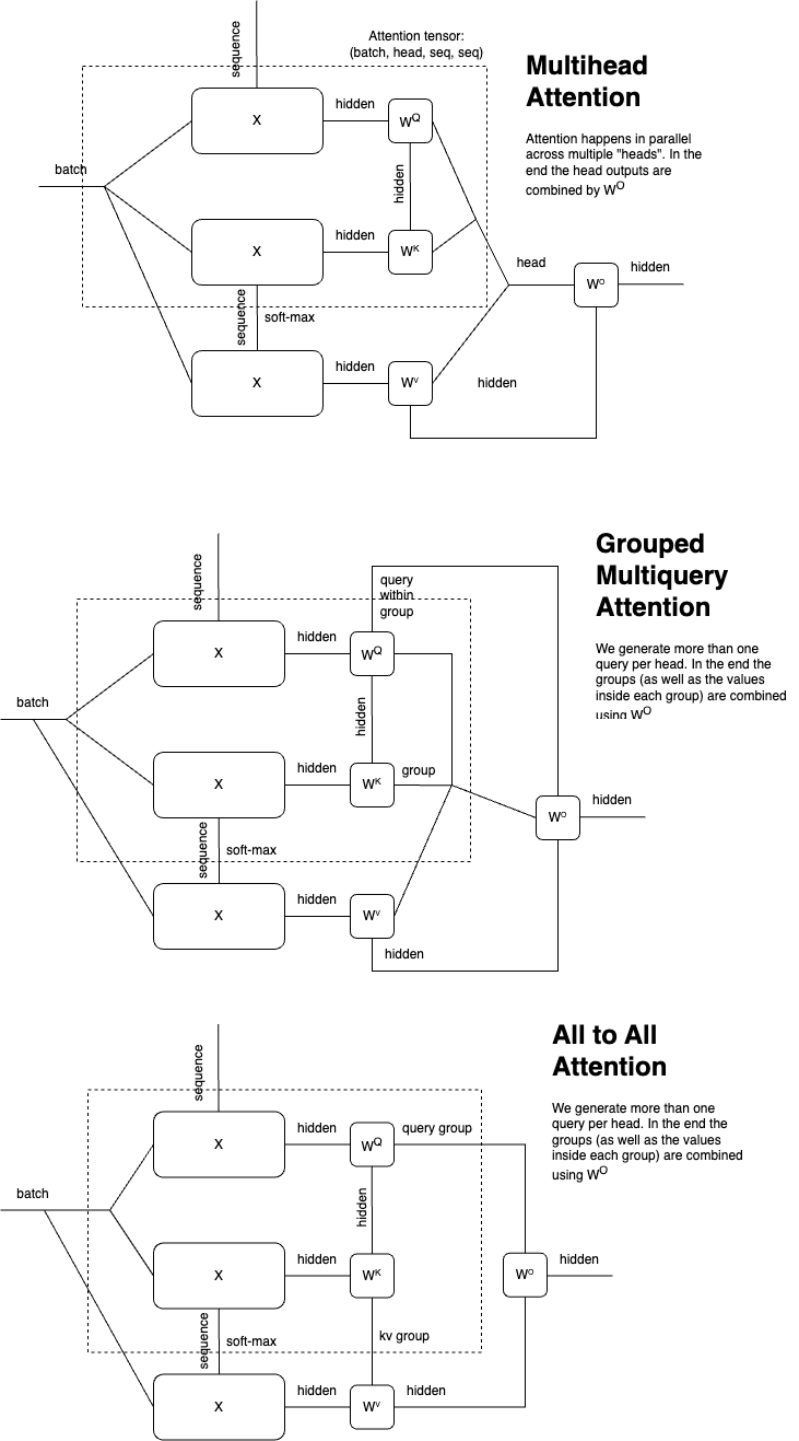
step = compile_to_callable(loss, *[loss.grad(p) for p in params], torch_compile=True)Because tensor edges have names, multi-head attention needs no
view/transpose gymnastics — heads are just an edge named head, and
attention keys are made by renaming seq to key:
att = F.softmax(F.dot(q, k, dim="hs") / math.sqrt(head_size) + causal_mask, dim="key")LayerNorm is written in three lines of mean/sqrt and its backward pass is
derived, token embeddings are a real integer F.gather (scatter-add
gradient included), and softmax comes out fused and numerically stabilized at
compile time.
from tensorgrad import Variable
import tensorgrad.functions as F

# Define sizes for the tensor edges and variables
b, x, y = sp.symbols("b x y")
X = tg.Variable("X", b, x)
Y = tg.Variable("Y", b, y)
W = tg.Variable("W", x, y)

# Define the error
error = X @ W - Y

# The Frobenius norm squared is just the contraction
# of the all the edges of the tensor with itself
loss = error @ error

# Compute the derivative of the loss wrt W
expr = tg.Derivative(loss, W)
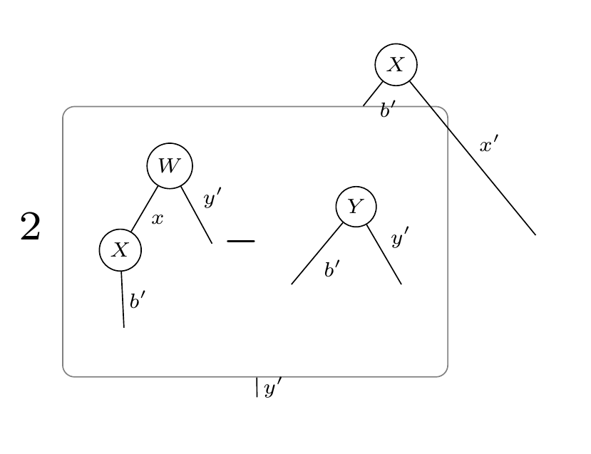
This will output the tensor diagram:
Tensorgrad can also compile the gradient to PyTorch code and show you exactly what it generated (verbose=True prints the kernel when it is first specialized to concrete sizes):
>>> from tensorgrad.compiler import compile_to_callable
>>> step = compile_to_callable(expr, verbose=True)
>>> grad_W = step({X: X_val, Y: Y_val, W: W_val}, {b: 128, x: 10, y: 5})
def _compiled(t1, t0, t3):                     # t1 = W, t0 = X, t3 = Y
    _e0 = torch.mm(t0, t1)                     # X @ W
    t4 = _e0 - t3                              # X @ W - Y
    _e1 = torch.mm(t0.transpose(-2, -1), t4)   # X.T @ (X @ W - Y)
    t6 = 2.0 * _e1
    return (t6,)
(memory-freeing dels and alias assignments elided from the printed kernel)
For a more complicated example, consider the following program for computing the Entropy of Cross Entropy Loss:
# Define the logits and targets as vectors
i = sp.symbols("i")
logits = tg.Variable("logits", i)
target = tg.Variable("target", i)

# Define the softmax cross-entropy loss
e = F.exp(logits)
softmax = e / F.sum(e)
ce = -target @ F.log(softmax)

# Compute the Hessian by taking the gradient of the gradient
H = ce.grad(logits).grad(logits)

display_pdf_image(to_tikz(H.full_simplify()))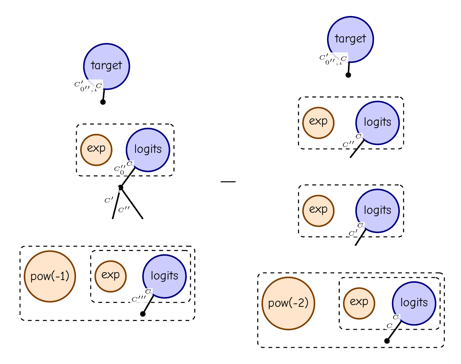
This is tensor diagram notation for (diag(p) - pp^T) sum(target), where p = softmax(logits).
Tensorgrad can also take expectations of arbitrary functions with respect to Gaussian tensors.
As an example, consider the L2 Loss program from before:
# Define sizes for the tensor edges and variables
b, x, y = sp.symbols("b x y")
X = tg.Variable("X", b, x)
Y = tg.Variable("Y", b, y)
W = tg.Variable("W", x, y)

# Define the mean and covariance variables of the distribution
mu = tg.Variable("mu", x, y)
# The coveriance of a matrix is a 4-tensor with two symmetries
C = tg.Variable("C", x, y, x2=x, y2=y).with_symmetries("x x2, y y2")

# Take the expectation of the L2 loss, assuming W ~ Normal(mu, C)
l2 = F.sum((X @ W - Y)**2)
E = tg.Expectation(l2, W, mu, C, covar_names={"x": "x2", "y": "y2"})

display_pdf_image(to_tikz(E.full_simplify()))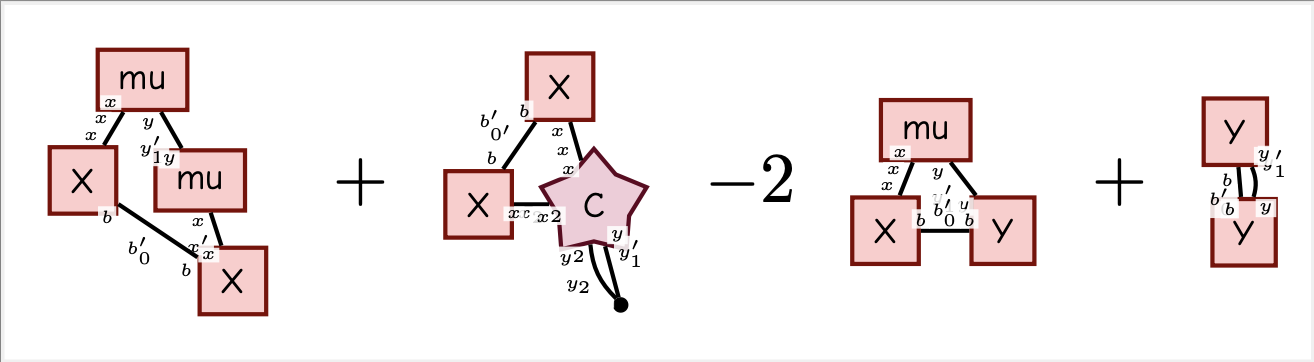
Note that the covariance is a rank-4 tensor (illustrated with a star) since we take the expectation with respect to a matrix. This is different from the normal "matrix shaped" covariance you get if you take expectation with respect to a vector.
Tensorgrad can evaluate your diagrams using PyTorch Named Tensors. It uses graph isomorphism detection to eliminate common subexpressions.
Tensorgrad can convert your diagrams back into pytorch code. This gives a super optimized way to do gradients and higher order derivatives in neural networks.
The ahead-of-time compiler (tensorgrad.compiler) turns a loss and its raw
symbolic gradients into one fused straight-line torch program:
from tensorgrad.compiler import compile_to_callable

step = compile_to_callable(loss, *[loss.grad(p) for p in params])
Primitives-defined layernorm/gelu gradients come out faster than torch autograd, convolutions 2–5x faster, and a 12-block GPT-2-sized gradient graph that would naively need exabytes of intermediates compiles to megabyte-scale nodes. Architecture, design principles, and benchmarks: docs/compiler.md.
In Penrose's book, The Road to Reality: A Complete Guide to the Laws of the Universe, he introduces a notation for taking derivatives on tensor networks. In this library we try to follow Penrose's notation, expanding it as needed to handle a full "chain rule" on tensor functions.

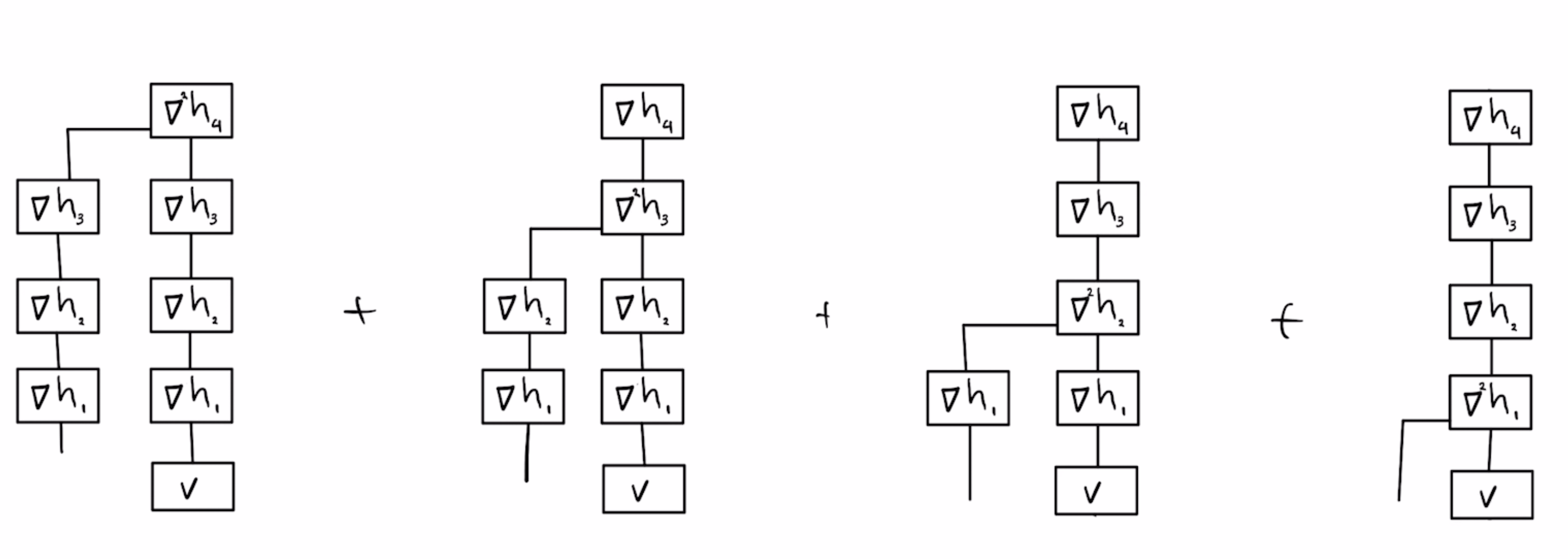
Another source of inspiration was Yaroslav Bulatov's derivation of the hessian of neural networks:
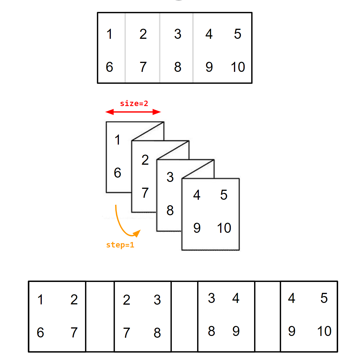
The main ingredient in CNNs are the linear operations Fold and Unfold. Unfold takes an image, with dimensions HxW and outputs P "patches" of size K^2, where K is the kernel size. Fold is the reverse operation. Since they are linear operations (they consist only of copying/adding) we can express them as a tensor with shape (H, W, P, K^2).
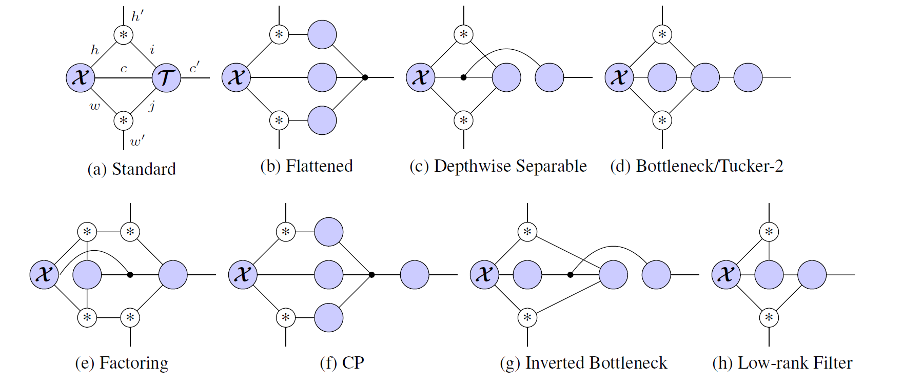
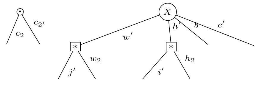
Hayashi et al. show that if you define a tensor (∗)_{i,j,k} = [i=j+k], then the "Unfold" operator factors along the spatial dimensions, and you can write a bunch of different convolutional neural networks easily as tensor networks:
With tensorgrad you can write the "standard" convolutional neural network like this:
data = Variable("data", ["b", "c", "w", "h"])
unfold = Convolution("w", "j", "w2") @ Convolution("h", "i", "h2")
kernel = Variable("kernel", ["c", "i", "j", "c2"])
expr = data @ unfold @ kernel
And then easily find the jacobian symbolically with expr.grad(kernel):
Taken from this Twitter thread: I wish I had known about Tensor Graphs back when I worked on Tensor-sketching. Let me correct this now and explain dimensionality reduction for tensors using Tensor Networks:
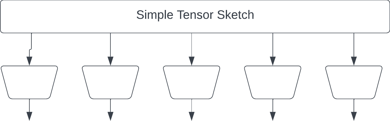
The second version is the "original" Tensor Sketch by Rasmus Pagh and Ninh Pham. (https://rasmuspagh.net/papers/tensorsketch.pdf) Each fiber is reduced by a JL sketch, and the result is element-wise multiplied. Note the output of each JL is larger than in the "simple" sketch to give the same output size.
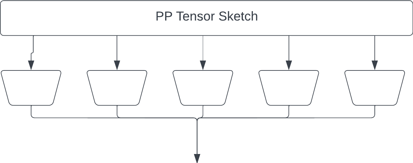
Next we have the "recursive" sketch by myself and coauthors in https://thomasahle.com/#paper-tensorsketch-joint. In the paper we sometimes describe this as a tree, but it doesn't really matter. We just had already created the tree-graphic when we realized.
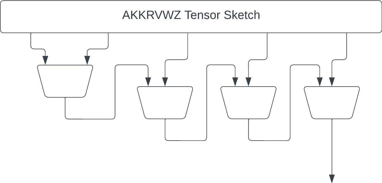
The main issue with the AKKRVWZ-sketch was that we used order-3 tensors internally, which require more space/time than simple random matrices in the PP-sketch. We can mitigate this issue by replacing each order-3 tensor with a simple order-2 PP-sketch.
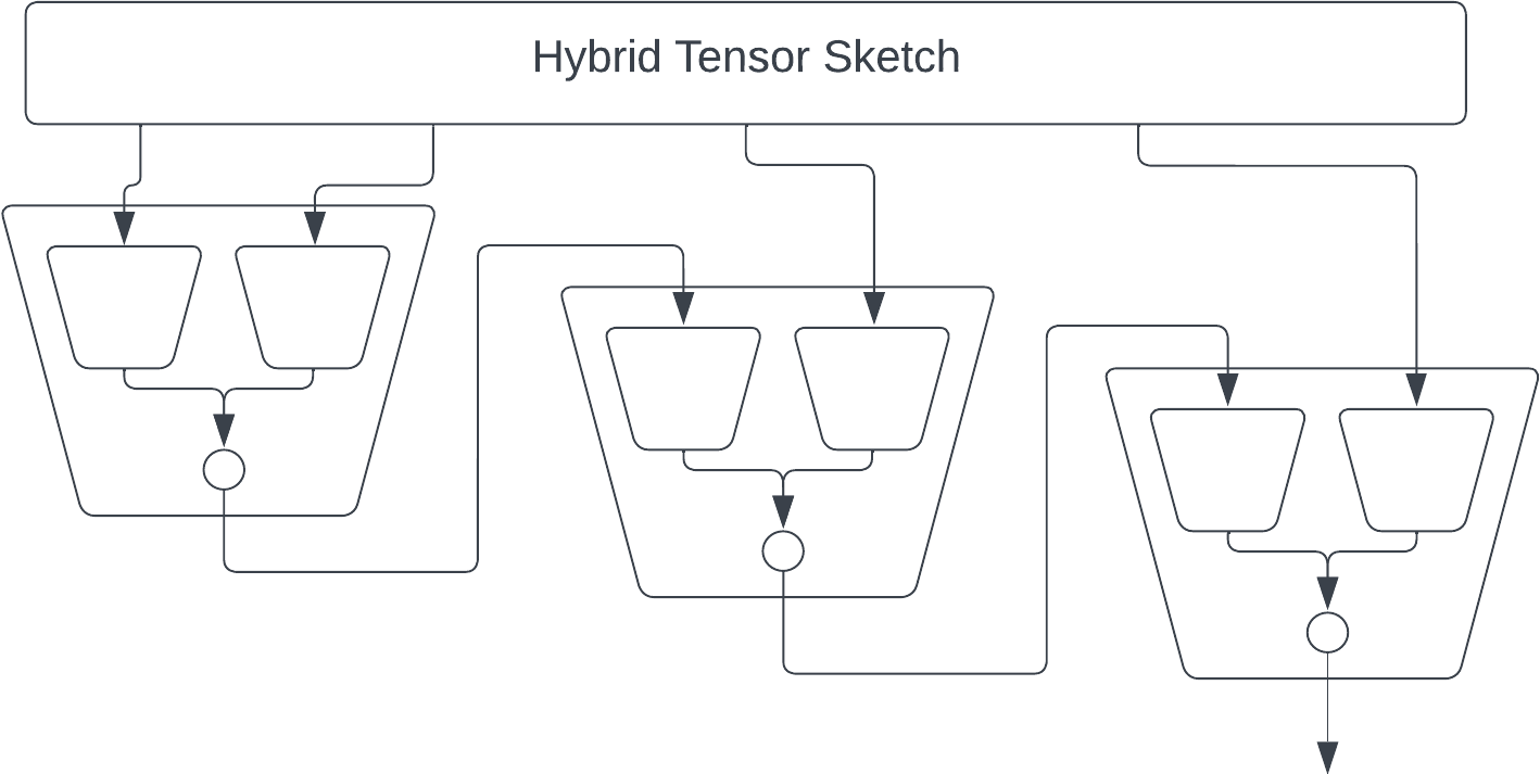
Finally we can speed up each matrix multiplication by using FastJL, which is itself basically an outer product of a bunch of tiny matrices. But at this point my picture is starting to get a bit overwhelming.
- Tool for creating tensor diagrams from einsum by Thomas Ahle
- Ideograph: A Language for Expressing and Manipulating Structured Data by Stephen Mell, Osbert Bastani, Steve Zdancewic